Vector search & kNN implementation guide - API edition

This guide focuses on setting up Elasticsearch for vector search and approximate k-nearest neighbor (kNN) search using the Elasticsearch APIs via HTTP or Python.

For users who will be primarily using Kibana, or wish to test through the UI, visit the Getting Started with semantic search guide using the Elastic crawler.

If you want to cut to the chase and just run some code in Jupyter Notebook, we have you covered with the accompanying notebook

Elastic Learned Sparse Encoder

If the text you are working with is English text, consider using the Elastic Learned Sparse Encoder

Elastic Learned Sparse EncodeR - or ELSER - is an NLP model trained by Elastic that enables you to perform semantic search by using sparse vector representation. Instead of literal matching on search terms, semantic search retrieves results based on the intent and the contextual meaning of a search query.

Otherwise, continue below for information on Semantic Vector search with approximate kNN search

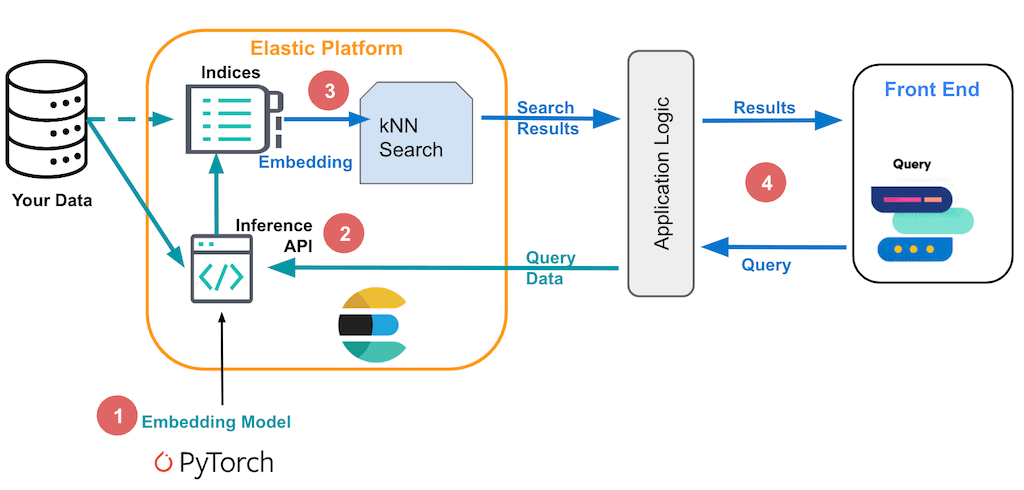
Vector search high-level architecture

There are four key components for implementing vector search in Elastic:

Embedding model: the machine learning model that takes your data as input and returns a numeric representation of the data (a vector, a.k.a. an “embedding”)
Inference endpoint: the Elastic Inference API or Elastic Inference pipeline processor that applies the machine learning model to text data. You use inference endpoints both when you ingest data and when you execute queries on the data. **NOTE: **for non-text data, such as image files, use an external script with your ML model in order to generate embeddings that you will store and use in Elastic.
Search: Elastic stores the embeddings along with your metadata in its indices, and then performs a (approximate) k-nearest neighbor search to find the closest matches of a query to your data (in vector space, a.k.a. “embedding space”)
Application logic: everything your application needs outside of the core vector search, such as communicating with users or applying your business logic.

Cluster considerations

Cluster sizing estimation

Memory considerations

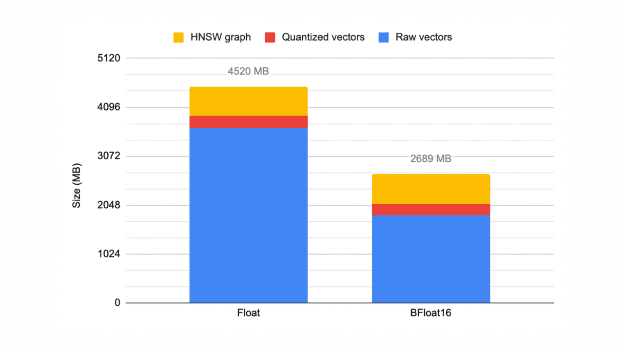
To be performant, vectors need to "fit" in off-heap RAM on the data nodes. As of Elasticsearch version 8.7+, the rough estimate required for vectors is

$NumVectors \times 4 \times (NumDimensions + 12)$

Note: this formula applies to Float type vectors.

quick example using 20 million vector fields (we'll assume 1 vector per document):

$20,000,000 \times 4 \times (768 +12) \approx 115\ GB\ of\ RAM\ off\ heap$

Note: Each replica added requires the same amount of additional RAM (eg. 1 primary and 1 replica for the example above, we estimate we would require 2x the RAM, or 230GB, for that estimate).

Performance testing

As every user's data is different the best approach for estimating RAM requirements is through testing. We recommend starting with a single node, single primary shard, no replica, and testing with that to find how many vectors "fit" on a node before performance drops off.

One way to accomplish this is with Elastic's benchmarking tool Rally.

If all the vectors are fairly small (eg. 3GB on a 64GB node), you can simply load the vectors and test in one shot to start.

Using the estimation formula above, load 75% of that number of vectors into a single node, run a challenge, and evaluate the response time metrics. Gradually increase the vector count, rerunning the tests, until performance drops below acceptable levels. The max count at which response times were acceptable can be considered generally the number of vectors for a single node. From there you can scale out nodes and replicas.

Jupyter notebook code

All the code below is available in a python Jupyter Notebook This code can be run entirely from the browser uding Google Colab for quick setup and testing using the accompanying notebook

Cluster configuration

Single vector per field vs multiple vectors per field

The standard approach to vector layout is one vector per field. This is the approach we will be following below. However, as of 8.11, Elasticsearch supports nested vectors which allow for multiple vectors per field. For information about setting up that approach check out the Elasticsearch Labs blog Chunking Large Documents via Ingest pipelines plus nested vectors equals easy passage search

Loading the embedding model

Embedding models run on Machine Learning nodes. Ensure you have one or more ML nodes deployed.

To load an embedding model into Elasticsearch, you will need to use Eland. Eland is a Python Elasticsearch client for exploring and analyzing data in Elasticsearch with a familiar Pandas-compatible API.

You can use Docker to quickly load a model from Hugging Face.
You can also use a jupyter notebook in Colab to quickly load a model (follow up through “Deploy an NLP model”)
For environments where you are unable to connect directly to Hugging Face, follow the steps outlined in the documentation Loading embedding model with Eland in an air-gapped environment

Ingest pipeline setup

There are multiple ways to generate an embedding for new documents. The simplest is to create an ingest pipeline and configure data targeted to an index to automatically use the pipeline to call the model with the inference processor.

In the example below we will create a pipeline with one processor, the inference processor. That processor will:

Map the field we want to create an embedding for, my_text, to the name the embedding model expects text_field in this case
Configure which model to use with model_id. This is the name of the model within Elasticsearch
Handle when any errors may occur for monitoring.

PUT _ingest/pipeline/vector_embedding_demo
{
  "processors": [
    {
      "inference": {
        "field_map": {
          "my_text": "text_field"
        },
        "model_id": "sentence-transformers__all-distilroberta-v1",
        "target_field": "ml.inference.my_vector",
        "on_failure": [
          {
            "append": {
              "field": "_source._ingest.inference_errors",
              "value": [
                {
                  "message": "Processor 'inference' in pipeline 'ml-inference-title-vector' failed with message '{{ _ingest.on_failure_message }}'",
                  "pipeline": "ml-inference-title-vector",
                  "timestamp": "{{{ _ingest.timestamp }}}"
                }
              ]
            }
          }
        ]
      }
    },
    {
      "set": {
        "field": "my_vector",
        "if": "ctx?.ml?.inference != null && ctx.ml.inference['my_vector'] != null",
        "copy_from": "ml.inference.my_vector.predicted_value",
        "description": "Copy the predicted_value to 'my_vector'"
      }
    },
    {
      "remove": {
        "field": "ml.inference.my_vector",
        "ignore_missing": true
      }
    }
  ]
}

Index mapping / template setup

Embeddings (vectors) are stored in the dense_vector field type in Elasticsearch. Next we will configure the index template before indexing documents and generating embeddings.

The below API call will create an index template to match any indices with the pattern my_vector_index-*

It will:

Configure dense_vector for my_vector as outlined in the documentation.
It is recommended to Exclude the vector field from _source
We will also include one text field, my_text in this example which will be the source the embedding is generated from.

PUT /_index_template/my_vector_index
{
  "index_patterns": [
    "my_vector_index-*"
  ],
  "priority": 1,
  "template": {
    "settings": {
      "number_of_shards": 1,
      "number_of_replicas": 1,
      "index.default_pipeline": "vector_embedding_demo"
    },
    "mappings": {
      "properties": {
        "my_vector": {
          "type": "dense_vector",
          "dims": 768,
          "index": true,
          "similarity": "dot_product"
        },
        "my_text": {
          "type": "text"
        }
      },
      "_source": {
        "excludes": [
          "my_vector"
        ]
      }
    }
  }
}

Indexing data

There are many ways to index data into Elasticsearch. The example below shows a quick set of test documents to be indexed into the example index. Embeddings will be generated in ingest by the ingest pipeline when the inference processor makes an internal API call to the embedding model.

POST my_vector_index-01/_bulk?refresh=true
{"index": {}}
{"my_text": "Hey, careful, man, there's a beverage here!", "my_metadata": "The Dude"}
{"index": {}}
{"my_text": "I’m The Dude. So, that’s what you call me. You know, that or, uh, His Dudeness, or, uh, Duder, or El Duderino, if you’re not into the whole brevity thing", "my_metadata": "The Dude"}
{"index": {}}
{"my_text": "You don't go out looking for a job dressed like that? On a weekday?", "my_metadata": "The Big Lebowski"}
{"index": {}}
{"my_text": "What do you mean brought it bowling, Dude? ", "my_metadata": "Walter Sobchak"}
{"index": {}}
{"my_text": "Donny was a good bowler, and a good man. He was one of us. He was a man who loved the outdoors... and bowling, and as a surfer he explored the beaches of Southern California, from La Jolla to Leo Carrillo and... up to... Pismo", "my_metadata": "Walter Sobchak"}

Querying data

Approximate k-nearest neighbor

GET my_vector_index-01/_search
{
  "knn": [
    {
      "field": "my_vector",
      "k": 1,
      "num_candidates": 5,
      "query_vector_builder": {
        "text_embedding": {
          "model_id": "sentence-transformers__all-distilroberta-v1",
          "model_text": "Watchout I have a drink"
        }
      }
    }
  ]
}

Hybrid searching (kNN + BM25) with Reciprocal rank fusion technical preview

GET my_vector_index-01/_search
{
  "size": 2,
  "query": {
    "match": {
      "my_text": "bowling"
    }
  },
  "knn":{
      "field": "my_vector",
      "k": 3,
      "num_candidates": 5,
      "query_vector_builder": {
        "text_embedding": {
          "model_id": "sentence-transformers__all-distilroberta-v1",
          "model_text": "He enjoyed the game"
        }
      }
    },
      "rank": {
        "rrf": {}
    }
}

Filtering

GET my_vector_index-01/_search
{
  "knn": {
    "field": "my_vector",
    "k": 1,
    "num_candidates": 5,
    "query_vector_builder": {
      "text_embedding": {
        "model_id": "sentence-transformers__all-distilroberta-v1",
        "model_text": "Did you bring the dog?"
      }
    },
    "filter": {
      "term": {
        "my_metadata": "The Dude"
      }
    }
  }
}

Aggregations with select fields returned

GET my_vector_index-01/_search
{
  "knn": {
    "field": "my_vector",
    "k": 2,
    "num_candidates": 5,
    "query_vector_builder": {
      "text_embedding": {
        "model_id": "sentence-transformers__all-distilroberta-v1",
        "model_text": "did you bring it?"
      }
    }
  },
  "aggs": {
    "metadata": {
      "terms": {
        "field": "my_metadata"
      }
    }
  },
  "fields": [
    "my_text",
    "my_metadata"
  ],
  "_source": false
}

kNN tuning options

An overview of tuning options is covered in the documentation Tune approximate kNN search

The computational cost of search: logarithmic in the number of vectors, provided they are indexed through HNSW. And slightly better than linear in the number of dimensions for dot_product similarity

_search

Tune approximate kNN for speed or accuracy Docs

Choice of distance metrics

Whenever possible, we recommend using dot_product instead of cosine similarity when deploying vector search to production. Using dot product avoids having to calculate the vector magnitudes for every similarity computation (because the vectors are normalized in advance to all have magnitude 1). This means it can improve search and indexing speed by ~2-3x.
That said, cosine is popular for text applications: the length of the query is typically much shorter than the ingested documents, so the distance to the original doesn’t meaningfully contribute to the measurement of similarity. Remember cosine requires 6 operations per tupel, whereas dot product only needs two for each dimension (multiply each element, then sum). Therefore we recommend using cosine only for testing/exploration and switching to dot product when you move to production (with normalizing, dot product will compute the cosine after all).
Try dot_product first in all other use cases - because its execution speed is so much faster than L2 norm (standard Euclidean).

Ingest

Indexing considerations Docs

Indexing new data

Unless you generate your own embeddings, you’ll have to generate embeddings for the new data upon ingestion. For text, that’s accomplished with an ingest pipeline with an inference processor calling a hosted embedding model. Note this requires a Platinum license.
Adding more data also increases RAM - since you need to keep all vectors off-heap (whereas with traditional search that would be disk)

Exact kNN search

aka Brute Force or Script Score

Exact kNN Search Docs

Don’t assume you need ANN because some use cases work fine without ANN. As a rule of thumb, if the number of documents you are actually ranking (i.e. after filters are applied) is under 10k, you are likely better off using a brute-force option

Elasticsearch is packed with new features to help you build the best search solutions for your use case. Dive into our sample notebooks to learn more, start a free cloud trial, or try Elastic on your local machine now.