Transaction sampling

Distributed tracing can generate a substantial amount of data. More data can mean higher costs and more noise. Sampling aims to lower the amount of data ingested and the effort required to analyze that data — all while still making it easy to find anomalous patterns in your applications, detect outages, track errors, and lower mean time to recovery (MTTR).

Elastic APM supports two types of sampling:

In head-based sampling, the sampling decision for each trace is made when the trace is initiated. Each trace has a defined and equal probability of being sampled.

For example, a sampling value of .2 indicates a transaction sample rate of 20%. This means that only 20% of traces will send and retain all of their associated information. The remaining traces will drop contextual information to reduce the transfer and storage size of the trace.

Head-based sampling is quick and easy to set up. Its downside is that it’s entirely random — interesting data might be discarded purely due to chance.

See Configure head-based sampling to get started.

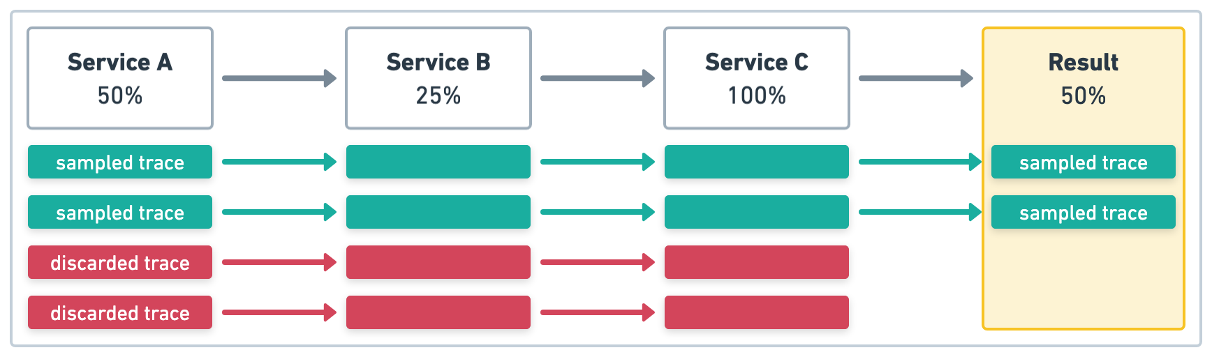
In a distributed trace, the sampling decision is still made when the trace is initiated. Each subsequent service respects the initial service’s sampling decision, regardless of its configured sample rate; the result is a sampling percentage that matches the initiating service.

In the example in Figure 1, Service A initiates four transactions and has sample rate of .5 (50%). The upstream sampling decision is respected, so even if the sample rate is defined and is a different value in Service B and Service C, the sample rate will be .5 (50%) for all services.

Figure 1. Upstream sampling decision is respected

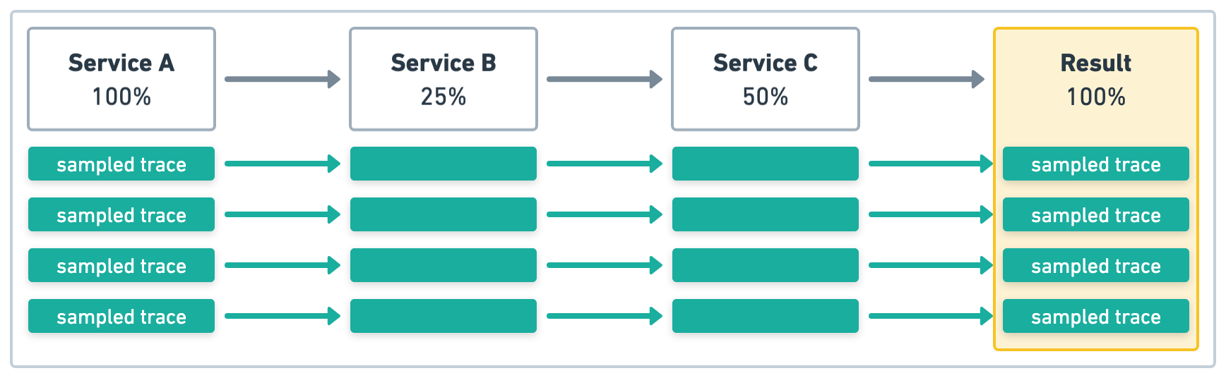
In the example in Figure 2, Service A initiates four transactions and has a sample rate of 1 (100%). Again, the upstream sampling decision is respected, so the sample rate for all services will be 1 (100%).

Figure 2. Upstream sampling decision is respected

In addition to setting the sample rate, you can also specify which trace continuation strategy to use. There are three trace continuation strategies: continue, restart, and restart_external.

The continue trace continuation strategy is the default and will behave similar to the examples in the Distributed tracing section.

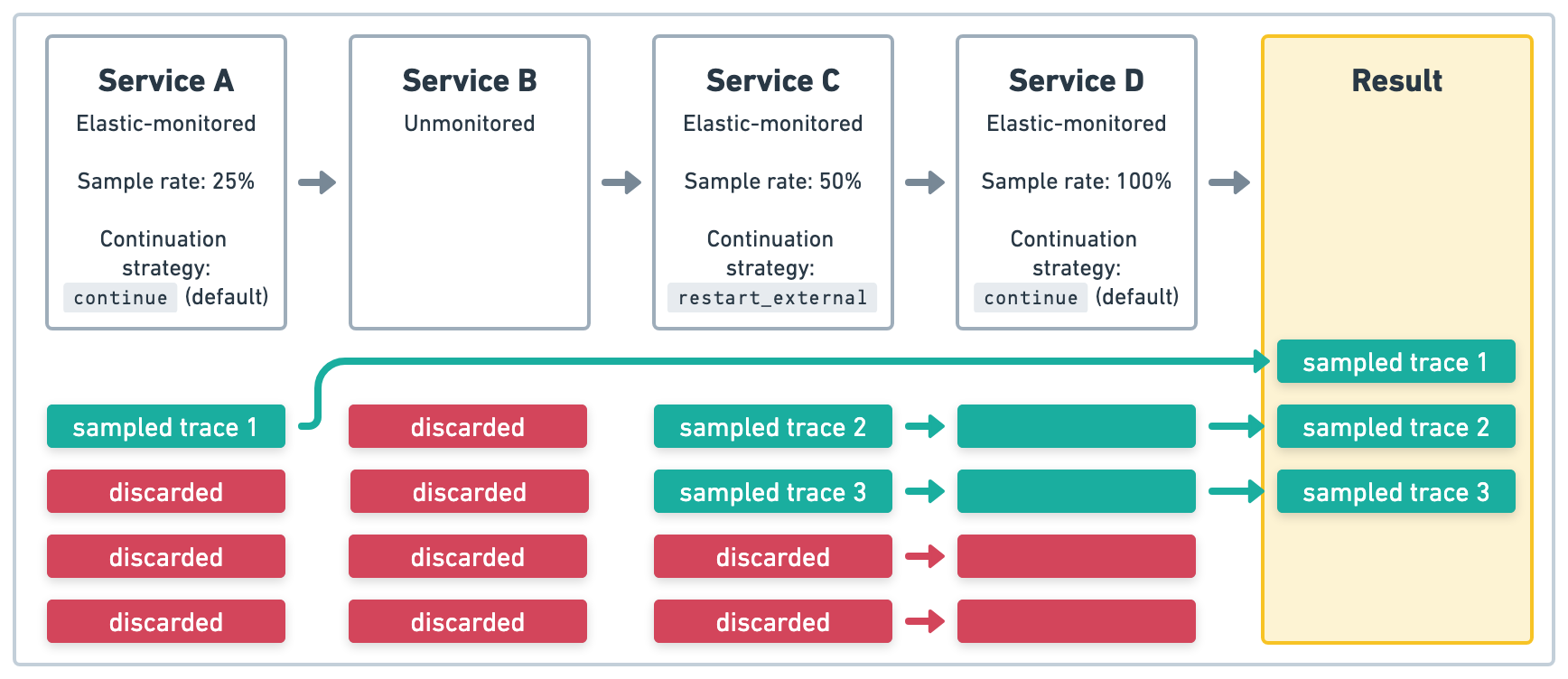
Use the restart_external trace continuation strategy on an Elastic-monitored service to start a new trace if the previous service did not have a traceparent header with es vendor data. This can be helpful if a transaction includes an Elastic-monitored service that is receiving requests from an unmonitored service.

In the example in Figure 3, Service A is an Elastic-monitored service that initiates four transactions with a sample rate of .25 (25%). Because Service B is unmonitored, the traces started in Service A will end there. Service C is an Elastic-monitored service that initiates four transactions that start new traces with a new sample rate of .5 (50%). Because Service D is also Elastic-monitored service, the upstream sampling decision defined in Service C is respected. The end result will be three sampled traces.

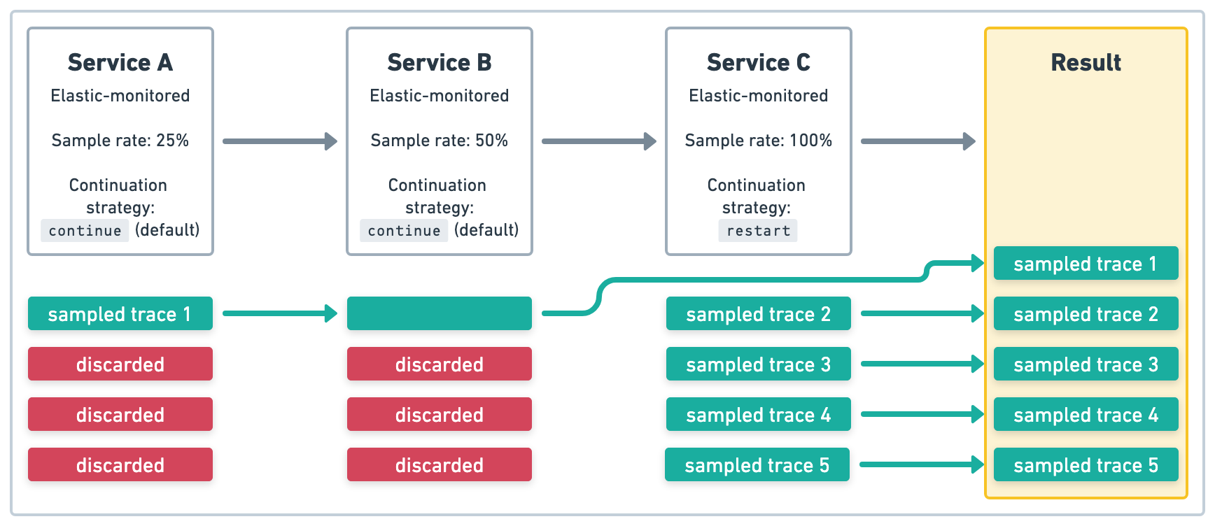
Figure 3. Using the restart_external trace continuation strategy

Use the restart trace continuation strategy on an Elastic-monitored service to start a new trace regardless of whether the previous service had a traceparent header. This can be helpful if an Elastic-monitored service is publicly exposed, and you do not want tracing data to possibly be spoofed by user requests.

In the example in Figure 4, Service A and Service B are Elastic-monitored services that use the default trace continuation strategy. Service A has a sample rate of .25 (25%), and that sampling decision is respected in Service B. Service C is an Elastic-monitored service that uses the restart trace continuation strategy and has a sample rate of 1 (100%). Because it uses restart, the upstream sample rate is not respected in Service C and all four traces will be sampled as new traces in Service C. The end result will be five sampled traces.

Figure 4. Using the restart trace continuation strategy

Head-based sampling is implemented directly in the APM agents and SDKs. The sample rate must be propagated between services and the managed intake service in order to produce accurate metrics.

OpenTelemetry offers multiple samplers. However, most samplers do not propagate the sample rate. This results in inaccurate span-based metrics, like APM throughput, latency, and error metrics.

For accurate span-based metrics when using head-based sampling with OpenTelemetry, you must use a consistent probability sampler. These samplers propagate the sample rate between services and the managed intake service, resulting in accurate metrics.

In tail-based sampling, the sampling decision for each trace is made after the trace has completed. This means all traces will be analyzed against a set of rules, or policies, which will determine the rate at which they are sampled.

Unlike head-based sampling, each trace does not have an equal probability of being sampled. Because slower traces are more interesting than faster ones, tail-based sampling uses weighted random sampling — so traces with a longer root transaction duration are more likely to be sampled than traces with a fast root transaction duration.

A downside of tail-based sampling is that it results in more data being sent from APM agents to the APM Server. The APM Server will therefore use more CPU, memory, and disk than with head-based sampling. However, because the tail-based sampling decision happens in APM Server, there is less data to transfer from APM Server to Elasticsearch. So running APM Server close to your instrumented services can reduce any increase in transfer costs that tail-based sampling brings.

See Configure tail-based sampling to get started.

Distributed tracing with tail-based sampling

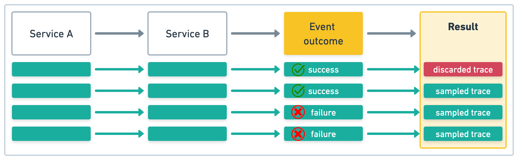
With tail-based sampling, all traces are observed and a sampling decision is only made once a trace completes.

In this example, Service A initiates four transactions. If our sample rate is .5 (50%) for traces with a success outcome, and 1 (100%) for traces with a failure outcome, the sampled traces would look something like this:

OpenTelemetry with tail-based sampling

Tail-based sampling is implemented entirely in APM Server, and will work with traces sent by either Elastic APM agents or OpenTelemetry SDKs.

Due to OpenTelemetry tail-based sampling limitations when using tailsamplingprocessor, we recommend using APM Server tail-based sampling instead.

A sampled trace retains all data associated with it. A non-sampled trace drops all span and transaction data¹. Regardless of the sampling decision, all traces retain error data.

Some visualizations in the APM app, like latency, are powered by aggregated transaction and span metrics. The way these metrics are calculated depends on the sampling method used:

For all sampling methods, metrics are weighted by the inverse sampling rate of the head-based sampling policy to provide an estimate of the total population. For example, if your head-based sampling rate is 5%, each sampled trace is counted as 20. As the variance of latency increases or the head-based sampling rate decreases, the level of error in these calculations may increase.

These calculation methods ensure that the APM app provides the most accurate metrics possible given the sampling strategy in use, while also accounting for the head-based sampling rate to estimate the full population of traces.

¹ Real User Monitoring (RUM) traces are an exception to this rule. The Kibana apps that utilize RUM data depend on transaction events, so non-sampled RUM traces retain transaction data — only span data is dropped.

What’s the best sampling rate? Unfortunately, there isn’t one. Sampling is dependent on your data, the throughput of your application, data retention policies, and other factors. A sampling rate from .1% to 100% would all be considered normal. You’ll likely decide on a unique sample rate for different scenarios. Here are some examples:

Regardless of the above, cost conscious customers are likely to be fine with a lower sample rate.