From vector search to powerful REST APIs, Elasticsearch offers developers the most extensive search toolkit. Dive into our sample notebooks in the Elasticsearch Labs repo to try something new. You can also start your free trial or run Elasticsearch locally today.
Introduction
As we have discussed previously in Scalar Quantization 101 most embedding models output vector values, which is often excessive to represent the vector space. Scalar quantization techniques greatly reduce the space needed to represent these vectors. We've also previously talked about Bit Vectors In Elasticsearch and how binary quantization can often be unacceptably lossy.
With binary quantization techniques such as those presented in the RaBitQ paper we can address the problems associated with naively quantizing into a bit vector and maintain the quality associated with scalar quantization by more thoughtfully subdividing the space and retaining residuals of the transformation. These newer techniques allow for better optimizations and generally better results over other similar techniques like product quantization (PQ) in distance calculations and a 32x level of compression that typically is not possible with scalar quantization.
Here we'll walk through some of the core aspects of binary quantization and leave the mathematical details to the RaBitQ paper.
Building the Bit Vectors
Because we can more efficiently pre-compute some aspects of the distance computation, we treat the indexing and query construction separately.
To start with let's walk through indexing three very simple 2 dimensional vectors, , , and , to see how they are transformed and stored for efficient distance computations at query time.
Our objective is to transform these vectors into much smaller representations that allow:
- A reasonable proxy for estimating distance rapidly
- Some guarantees about how vectors are distributed in the space for better control over the total number of data vectors needed to recall the true nearest neighbors
We can achieve this by:
- Shifting each vector to within a hyper-sphere, in our case a 2d circle, the unit circle
- Snapping each vector to a single representative point within each region of the circle
- Retaining corrective factors to better approximate the distance between each vector and the query vector
Let's unpack that step by step.
Find a Representative Centroid
In order to partition each dimension we need to pick a pivot point. For simplicity, we'll select one point to use to transform all of our data vectors.
Let's continue with our vectors, , , and . We pick their centroid as the pivot point.
Here's all of those points graphed together:
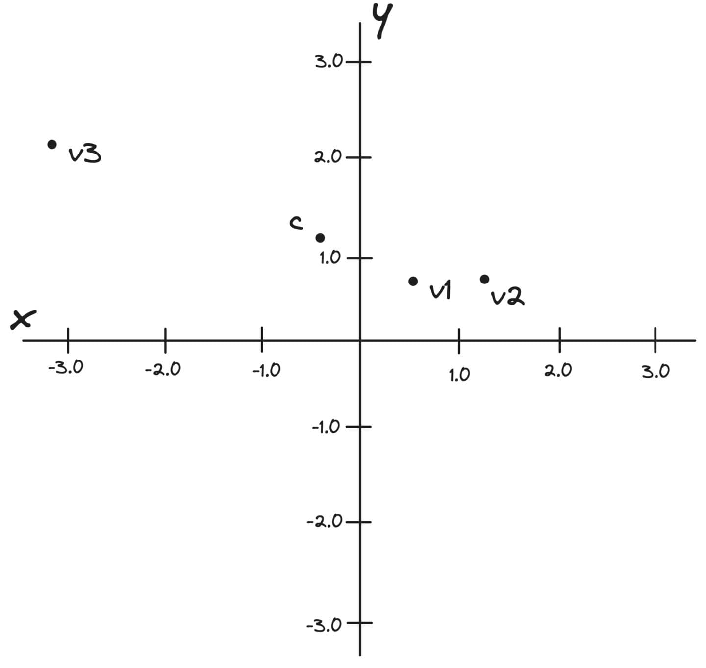
Figure 1: graph of the example vectors and the derived centroid of those three vectors.
Each residual vector is then normalized. We'll call these , , and .
Let's do the math for one of the vectors together:
And for each of the remaining vectors:
Let's see that transformation and normalization all together:
Figure 2: Animation of the example vectors and the derived centroid transformed within the unit circle.
As you may be able to see our points now sit on the unit circle around the centroid as if we had placed the centroid at 0,0.
1 Bit, 1 Bit Only Please
With our data vectors centered and normalized, we can apply standard binary quantization encoding each transformed vector component with a 0 if it is negative and 1 if it is positive. In our 2 dimensional example this splits our unit circle into four quadrants and the binary vectors corresponding to , , and become , respectively.
We finish quantizing each data vector by snapping it to a representative point within each region specifically picking a point equidistant from each axis on the unit circle:
We'll denote each quantized vector as , , and .
So for instance if we snap to its representative point within its region we get:
And here are the quantized forms for the other data vectors, and :
Picking these representative points has some nice mathematical properties as outlined in the RaBitQ paper. And are not unlike the codebooks seen in product quantization (PQ).
Figure 3: Binary quantized vectors within a region snapped to representative points.
At this point we now have a 1 bit approximation; albeit a somewhat fuzzy one that we can use to do distance comparisons. Clearly, and are now identical in this quantized state, which is not ideal and is a similar problem experienced when we discussed encoding float vectors as Bit Vectors In Elasticsearch.
The elegance of this is that at query time we can use something akin to a dot product to compare each data vector and each query vector rapidly for an approximation of distance. We'll see that in more detail when we discuss handling the query.
The Catch
As we saw above, a lot of information is lost when converting to bit vectors. We'll need some additional information to help compensate for the loss and correct our distance estimations.
In order to recover fidelity we'll store the distance from each vector to the centroid and the projection (dot product) of the vector (e.g ) with its quantized form (e.g. ) as two values.
The Euclidean distance to the centroid is straight-forward and we already computed it when quantizing each vector:
Precomputing distances from each data vector to the centroid restores the transformation of centering the vectors. Similarly, we'll compute the distance from the query to the centroid. Intuitively the centroid acts as a go-between instead of directly computing the distance between the query and data vector.
The dot product of the vector and the quantized vector is then:
And for our other two vectors:
The dot product between the quantized vector and the original vector, being the second corrective factor, captures for how far away the quantized vector is from its original position. In section 3.2 the RaBitQ paper shows there is a bias correcting the dot product between the quantized data and query vectors in a naive fashion. This factor exactly compensates it.
Keep in mind we are doing this transformation to reduce the total size of the data vectors and reduce the cost of vector comparisons. These corrective factors while seemingly large in our 2d example become insignificant as vector dimensionality increases. For example, a 1024 dimensional vector if stored as requires 4096 bytes. If stored with this bit compression and corrective factors, only 136 bytes are required.
To better understand why we use these factors refer to the RaBitQ paper. It gives an in-depth treatment of the math involved.
The Query
To be able to compare our quantized data vectors to a query vector we must first get the query vector into a quantized form and shift it relative to the unit circle. We'll refer to the query vector as , the transformed vector as , and the scalar quantized vector as .
Next we perform Scalar Quantization on the query vector down to 4 bits; we'll call this vector . It's worth noting that we do not quantize down to a bit representation but instead maintain an scalar quantization, as an int4 byte array, for estimating the distance. We can take advantage of this asymmetric quantization to retain more information without additional storage.

Figure 4: Query with centroid transformation applied.
As you can see because we have only 2 dimensions our quantized query vector now consists of two values at the ceiling and floor of the range. With longer vectors you would see a variety of int4 values with one of them being the ceiling and one of them being the floor.
Now we are ready to perform a distance calculation comparing each indexed data vector with this query vector. We do this by summing up each dimension in our quantized query that's shared with any given data vector. Basically, a plain old dot-product, but with bits and bytes.
We can now apply corrective factors to unroll the quantization and get a more accurate reflection of the estimated distance.
To achieve this we'll collect the upper and lower bound from the quantized query, which we derived when doing the scalar quantization of the query. Additionally we need the distance from the query to the centroid. Since we computed the distance between a vector and a centroid previously we'll just include that distance here for reference:
Estimated Distance
Alright! We have quantized our vectors and collected corrective factors. Now we are ready to compute the estimated distance between and . Let's transform our Euclidean distance into an equation that has much more computationally friendly terms:
In this form, most of these factors we derived previously, such as , and notably can be pre-computed prior to query or are not direct comparisons between the query vector and any given data vector such as .
We however still need to compute . We can utilize our corrective factors and our quantized binary distance metric to estimate this value reasonably and quickly. Let's walk through that.
Let's start by estimating which requires this equation which essentially unrolls our transformations using the representative points we defined earlier:
Specifically, maps the binary values back to our representative point and undoes the shift and scale used to compute the scalar quantized query components.
We can rewrite this to make it more computationally friendly like this.
First, though, let's define a couple of helper variables:
- total number of 1's bits in as , in this case
- total number of all quantized values in as , in this case
With this value and , which we precomputed when indexing our data vector, we can then plug those values in to compute an approximation of :
Finally, let's plug this into our larger distance equation noting that we are using an estimate for :
With all of the corrections applied we are left with a reasonable estimate of the distance between two vectors. For instance in this case our estimated distances between each of our original data vectors, , , , and compared to the true distances are:
For details on how the linear algebra is derived or simplified when applied refer to the RaBitQ paper.
Re-ranking
As you can see from the results in the prior section, these estimated distances are indeed estimates. Binary quantization produces vectors whose distance calculations are, even with the extra corrective factors, only an approximation of the distance between vectors. In our experiments we were able to achieve high recall by involving a multi-stage process. This confirms the findings in the RaBitQ paper.
Therefore to achieve high quality results, a reasonable sample of vectors returned from binary quantization then must be re-ranked with a more exact distance computation. In practice this subset of candidates can be small achieving typically high > 95% recall with 100 or less candidates for large datasets (>1m).
With RaBitQ results are re-ranked continually as part of the search operation. In our experiments to achieve a more scalable binary quantization we decoupled the re-ranking step. While RaBitQ is able to maintain a better list of top candidates by re-ranking while searching, it is at the cost of constantly paging in full vectors, which is untenable for some larger production-like datasets.
Conclusion
Whew! You made it! This blog is indeed a big one. We are extremely excited about this new algorithm as it can alleviate many of the pain points of Product Quantization (e.g. code-book building cost, distance estimation slowness, etc.) and provide excellent recall and speed.
Frequently Asked Questions
What are the benefits of binary quantization?
Quantization allows for vectors to be encoded in a lossy manner, thus reducing fidelity slightly with huge space savings.
How does binary quantization work?
Binary quantization takes each vector and transforms it relative to a prototypical set of sample vectors creating a smaller representation that can be used to approximate distances at great space and computation savings.
Does binary quantization create codebooks similar to PQ?
Binary quantization does not really create codebooks and instead compresses each data vector down to a 1 bit representation that is the inclusion in a region around a centroid. The authors of the RaBitQ paper (https://arxiv.org/pdf/2405.12497), that is a large driver for our understanding and implementation of binary quantization, mention how the codebooks in PQ are related to the regions around any given centroid so if it's more intuitive to think of these regions as codebooks then yes.
Are the query vectors converted to 1 bit prior to comparison with the codebook / regions created from the data vectors?
Binary quantization relies on finding regions first. Query vectors similarly are transformed into this space using the same centroid that allowed transformation into the region that was used to quantize the data vectors. This is what allows the distance estimation comparison to happen.
Are there multiple centroids?
Yes, if the number of vectors justifies it. Although, even for millions of vectors, we have found that only one centroid is sufficient for many datasets and models.
Are the centroids converted to a 1 bit representation as well?
No, since very few centroids are required they can be maintained in their float32 form without concern for scaling.
The author's of the RaBitQ paper (https://arxiv.org/pdf/2405.12497) mention transforming the data with a random orthogonal matrix P why do you not include it here?
We've found so far that we can reduce complexity, both algorithmically and performance-wise, by removing this random transformation. While some vectors may be favored, traditionally reranking a reasonable set of data, which is required to achieve reasonable recall, seems to negate the need for this in practice.
The author's of the RaBitQ paper (https://arxiv.org/pdf/2405.12497) mention using multiple centroids but you focus on a single centroid here. Why only one centroid?
We've found so far that a single centroid for most production datasets works well. Additionally when talking about how binary quantization works we can focus on a single centroid at a time. As you have more vectors, >100m, you may find that recall is impacted. When using Elasticsearch these large datasets can be pre-partitioned and multiple centroids will naturally be used.
Related Content
February 16, 2026
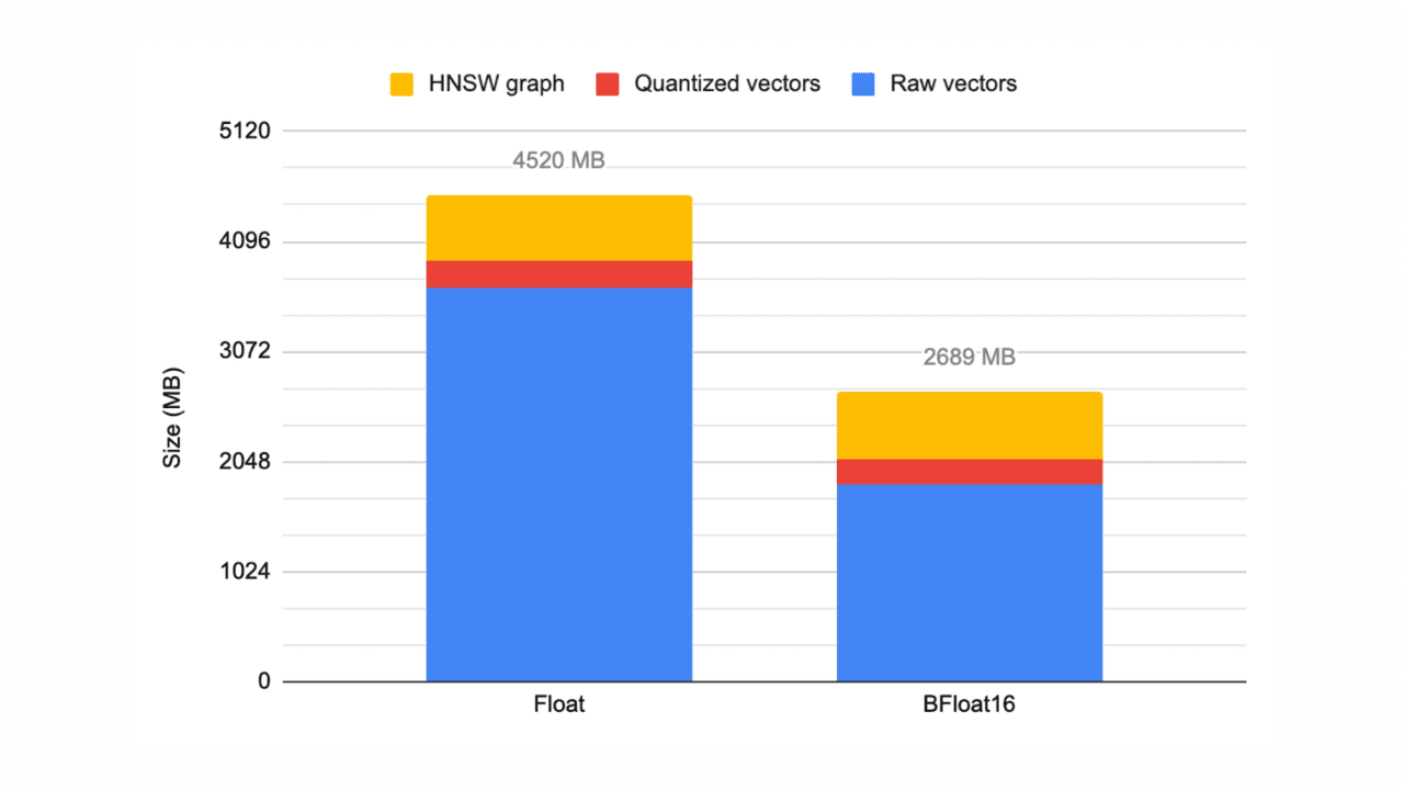
Elasticsearch 9.3 adds bfloat16 vector support
Exploring the new Elasticsearch element_type: bfloat16, which can halve your vector data storage.
February 10, 2026
How to defend your RAG system from context poisoning
How context engineering techniques prevent context poisoning in LLM responses.
February 4, 2026
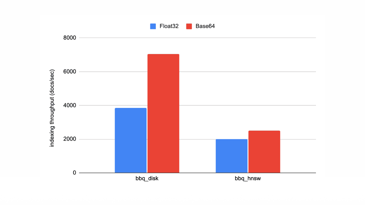
Speed up vector ingestion using Base64-encoded strings
Introducing Base64-encoded strings to speed up vector ingestion in Elasticsearch.

February 5, 2026
ES|QL dense vector search support
Using ES|QL for vector search on your dense_vector data.

January 28, 2026
Apache Lucene 2025 wrap-up
2025 was a stellar year for Apache Lucene; here are our highlights.