From vector search to powerful REST APIs, Elasticsearch offers developers the most extensive search toolkit. Dive into our sample notebooks in the Elasticsearch Labs repo to try something new. You can also start your free trial or run Elasticsearch locally today.
Vector databases are quickly becoming the de facto data store for semantic search, a type of search that considers context and meaning of content over traditional keyword search. Elastic has consistently provided modern tooling to perform semantic search, and it is important to identify and understand the larger mechanisms required to query a vector database.
This article will cover the necessary components to operate a vector database within Elasticsearch. We will explore the underlying technologies to create an efficient system to ensure the best performance and speed balance. Topics covered include:
- Current Elastic Full-Text Search ( BM25 & TF/IDF )
- Vectors, Embedding, and necessary Considerations
- Choosing an Embedding Model
- Indexing a Vector
- Vector Query Algorithms

Running the code to create your own vector database
To create your own vector database as shown within this article, you’ll need an
- Elasticsearch instance optimized for machine learning (8.13 or later)
- Docker Desktop or a similar Docker container manager
- Python 3.8 (or later)
- Elasticsearch Python Client
An associated repository is available here to illustrate the various moving parts necessary for querying a vector database. We will observe code snippets throughout the article from this source. The example repository will create an index of approximately 10,000 objects supplied in a JSON file representing science fiction books reviewed on goodreads.com. Each object will have a vector embedding of text that describes the book. The goal of this article and repository is to demonstrate searching for books based on vector similarity between a provided query string and the embedded book description vectors.
Here is a sample book object that we will be using within our code samples.
Current Elastic full-text search ( BM25 & TF/IDF )
To understand the scope and benefit of vector databases over traditional full-text search databases, it is worth taking a moment to review the current underlying technology that powers Elasticsearch, BM25, and its predecessor, TF/IDF.
TF/IDF
TF/IDF is the statistical measure of the frequency and importance of a query term based on how often it appears in an individual document and its rate of occurrence within an entire index of documents.
- Term Frequency (TF): This is a measure of how often a term occurs within a document. A higher occurrence of the term within a document, the higher the likelihood that the document will be relevant to the original query. This is measured as a raw count or normalized count based on the occurrence of the term divided by the total number of terms in the document
- Inverse Document Frequency (IDF): This is a measure of how important a query term is based on the overall frequency of use over all documents in an index. A term that occurs across more documents is considered less important and informative as is thus given less weight in the scoring. This is calculated as the logarithm of the total documents divided by the number of documents that contain the query term.
- nₜ = number of documents containing the term
- N = total number of documents
Using our example of Science Fiction books, lets break down a few sentences with a focus on the words "space" and "whales".
- "The interstellar whales graceully swam through the cosmos onto their next adventure."
- "The space pirates encountered a human space station on their trip to Venus, ripe for plunder"
- "In space no one can year you scream."
- "Space is the place to be."
- "Purrgil were a semi-sentient species of massive whales that lived in deep space, traveling from star system to star system."
Space
- The term "space" appears in 4 documents (Sentences 2, 3, 4, and 5).
- Total number of documents (N) = 5.
IDF formula for “space”:
"space" is considered less important because it appears frequently across 4 of the 5 sentences.
Whales
- The term "whales" appears in 2 documents (Sentences 1 and 5).
- Total number of documents (N) = 5.
IDF formula for “whales”:
"Whales" is considered relatively important because it appears in only 2 of 5 sentences.
"Whales" is assigned a higher IDF value because it appears in fewer documents, making it more distinctive and relevant to the context of those documents. Conversely, "space" is more common across the documents, leading to a lower IDF score, thus indicating that it is less useful for distinguishing between the documents. In the context of our codebase's 10,000 book ojbjects, the term "space" occurs 1,319 times, while the term "whale" appears 6 times total. It is understandable that a search for "space whales" would first prioritize the occurence of "whales" as more important than "space."
While still considered a powerful search algorithm in its own right, TF/IDF fails to prevent search bias on longer documents that may have a proportionately larger amount of term occurrences compared to a smaller document.
BM25
BM25 (Best Match 25) is an enhanced ranking function using IDF components to create a score outlining the relevance of a document over others within an index.
- Term Frequency Saturation: It has been noted that at a certain point, having a high occurrence of a query term in a document does not significantly increase its relevance compared to other documents with a similarly high count. BM25 introduces a saturation parameter for term frequency, which reduces the impact of the term frequency logarithmically as the count increases. This prevents very large documents with high term occurrences from disproportionately affecting the relevance score, ensuring that all scores level off after a certain point.
- Enhanced Inverse Document Frequency (IDF): In cases where a query term appears in all documents or has a very low occurrence, the IDF score might become zero. To avoid this, BM25 adds a value of 0.5 to the calculation, ensuring that the IDF scores do not reach zero or become too low.
- Average Document Length: This is a consideration of the actual length of the document. It's understood that longer documents may naturally have more occurrences of a term compared to shorter documents, which doesn't necessarily mean they are more relevant. This adjustment compensates for document length to avoid a bias towards longer documents simply due to their higher term frequencies.
BM25 is an excellent tool for efficient search and retrieval of exact-matches with text. Since 2016 it has been the default search algorithm for Lucene (versions 6.0 and higher), the underlying low-level search engine used by Elasticsearch. It should be noted that BM25 cannot provide semantic search as with vectors, which provides an understanding of the context of the query, rather than pure keyword search. It should also be noted that vocabulary mismatch may cause issues with receiving proper results. As an example, a user-submitted query using the term "cosmos" may not retrieve the intended results if the words don't exactly match, such as documents containing the term "space." It is understood that "cosmos" is another term for "space", but this isn't explicity known or checked for with the default BM25f algorithm. Knowing when to choose traditional keyword search over semantic search is crucial to ensure efficient use of computational resources.
Running the code: A full-text search (BM25)
Further Reading:
- The BM25 Algorithm and its variables
- BM25: A Guide to Modern Information Retrieveal
- BM25 The Next Generation of Lucene Relevance
Vectors & vector databases
Vector databases essentially store and index mathematical representations (vectors) of documents for similarity search. Vectorization of data allows for a normalization of complex and nuanced documents (text, images, audio, video, etc.) into a format that computers may compare with other vectors with consistent similarity results. It is important to understand the many mechanisms in place to provide a production-ready solution.
What is a vector?
A vector is a representation of data information projected into the mathematical realm as an array of numbers. With numbers instead of words, comparisons are very efficient for computers and thus offer a considerable performance boost. Nearly every conceivable data type (text, images, audio, video, etc.) used in computing may be converted into vector representations.
Images are broken down to the pixel and visual patterns such as textures, gradients, corners, and transparencies are captured into numeric representations. Words, words in specific phrases, and entire sentences are also analyzed, assigned various sentiment, contextual, and synonym values and converted to arrays of floating points. It is within these multidimensional matrices where systems are able to discern numeric similarities in certain portions of the vector to find similarly colored inventory in commerce sites, answers to coding questions on Elastic.co, or recognize the voice of a Nobel Prize winner.
Each data type benefits from a dedicated Vector Embedding Model, which can best identify and store the various characteristics of that particular type. A text embedding model excels at understanding common phrases and nuanced alliteration, while completely failing to recognize the emotions displayed on a posing figure in an image.

Above we can see the embedding model receiving three different strings as input and producing three distinct vectors (arrays of floats) as output.
Embedding models
When converting a vector of data, in this case, text, a model is used. It should be noted that models An embedding model is a pre-trained machine-learning instance that converts text (words, phrases, and sentences) into numerical representations. These representations become multidimensional arrays of floats, with each dimension representing a different characteristic of the original text, such as sentiment, context, and syntactics. These various representations allow for comparison with other vectors to find similar documents and text fragments.
Different embedding models have been developed that provide various benefits; some are extremely hardware efficient and can be run with less computational power. Some have a greater “understanding” of the context and content within the index it is storing within and can answer questions, perform text summarization, and lead a threaded conversation. Some focus on having an acceptable balance of performance and speed and efficiency.
Choosing an embedding model
We will briefly describe three models for text embeddings and their various properties.
Word2Vec: Efficient and simple to train, this model provides good quality embeddings for words based on their context as well as semantic meanings. Word2VEc is best used in applications with semantic similarly needs, sentiment analysis, or when computational resources are limited.
GloVe: Similar to Word2Vec in many respects, GloVe builds a global awareness across an entire index. By analyzing word co-occurrences throughout the entire text, GloVe captures both the frequency and context of words, resulting in embeddings that reflect the overall relationships and meanings of words in the totality of the stored vectors.
BERT: Unlike Word2Vec and GloVe, BERT (Bidirectional Encoder Representations from Transformers) looks at the text before and after each word to establish a local context and semantic meaning. By pre-training this model on a large body of text, this model excels at facilitating question and answer tasks as well as sentiment analysis.
Running the code: Creating an ingest pipeline to embed vectors
For the coding example, a smaller, simpler version of BERT was chosen called sentence-transformers__msmarco-minilm-l-12-v3. It is considered a MiniLM, which is more efficient than normal sized models yet still retains the performance needed for vector similarity. This is a good model choice for a non-production tutorial to get the code running quickly with no necessary fine tuning. More information about the model is available here
Below we are creating an ingest pipeline for our index books. This means that all book objects that are created and stored in the Elasticsearch index will automatically have their book_description field converted to a vector embedding named description_embedding. This reduces the codebase necessary to create new book objects on the client side.
If there is a failure, the documents will be stored in the failure-books index and an error message will be included in the documents. This allows you to view any errors that may have caused the failed embedding, and the ability to re-index the failed-index with updated code, ensuring no documents are lost or left behind.
Note: Since the workload of embedding the vectors is passed on to Elastic via this Inference Ingest Pipeline, it should be noted that a larger tier of available CPU and RAM in this Elasticsearch cloud instance may be desirable to allow for quick embedding and indexing of new and updated documents. If the workload of embedding is left to a local application codebase, consideration should also be given to the necessary compute hardware during times of high throughput. The provided codebase for this article includes an option to embed the book_description locally to allow for comparison and compute pressure.This snippet is creating an ingest pipeline named text-embedding which creates an inference processor. The processor uses the sentence-transformers__msmarco-minilm-l-12-v3 model to copy and convert the book_description text to a vector embedding and stores it under the description_embedding property.
Indexing vectors
The method in which vectors are indexed has a significant impact on the performance and accuracy of search results. Indexing vectors entails storing them in specialized data structures designed to ensure efficient similarity search, speedy vector distance calculations, and ultimately vector retrievals as results. How you decide to store your vectors should be based on your unique data needs. It should also be noted that Elasticsearch uses the term index as a verb acted upon documents to mean adding a document to an index. Care should be taken so as to not confuse the two.
There are two general methods of indexing documents: KNN, and ANN. It is important to make the distinction between the two and the tradeoffs when selecting one or the other.
KNN

Given k=4, four of the nearest vectors to the query vector (yellow) are selected and returned.
KNN (K-Nearest Neighbors) will provide an exact result of the K closest neighbor vectors based on a provided distance metric. As with most things that return exact results, the tradeoff is speed, which must be sacrificed for accuracy. The KNN method collates every distance from a target point to all other existing points in a dimension of a vector. The distances are then sorted and the closest K are returned. In the diagram above, a k of 4 is requested and the four nearest vectors are returned
ANN
ANN (Approximate Nearest Neighbors) will provide an approximation of the nearest neighbors based on an established index of vectors that have had their dimensions lowered for easier and faster processing. The tradeoff is a sped-up seeking phase where traversal is aided by an index, which could be thought of as a predefined map of all the vectors. ANN is preferred over KNN in semantic search when speed, scalability, and resource efficiency are considered higher priority over exact precision. This makes ANN a practical choice for large-scale and real-time applications where fast, approximate matches are acceptable. Much like a Probablistic Data Structure, a slight hit to accuracy has been accepted for the sake of speed and size.
As an example, think of various vector points being stored in shelves in a grocery store and you are given a map when you enter the facility. A premade map would allow you to find where you want to go vs traversing every single aisle from entrance to exit until you finally reach your intended point (KNN).
HNSW
HNSW (Hierarchical Navigable Small World) is the default ANN method with Elastic Vector Databases. It utilizes graph-based relationships (nodes and vertices) to efficiently traverse an index to find the nearest neighbors. In this case, the nodes are data points and the edges are connections to nearby neighbors. HNSW consists of many layers of graphs that have closer and closer distances to each other.

With HNSW, each subsequent traversal to a higher layer exposes closer nodes, or vectors, until the desired vector(s) are found.
This is similar to a traditional skip list data structure, where the higher layers have elements that are more far apart from each other, or “coarse” granularity, whereas the lower layers have elements that are closer to each other, or “finer” granularity. The traversal from a higher to lower plane of nodes and vertices means that not all vectors need to be searched and compared, only the nearest neighbors. This ensures that high dimensional vectors can be indexed and searched quickly and efficiently.
HNSW is ideally used for real-time semantic search and recommendation systems that have high-dimensional vectors yet can accept approximate results over exact nearest neighbors. HNSW can be considered extraneous with smaller data sets, lower-dimensional vectors, or when memory size-constraints are a factor. Due to the complexity of the graph structure, HNSW may not be a good fit for a highly dynamic data store where inserts, updates, and deletions occur in high frequency. This is due to the overhead maintenance of the graph connections throughout the many different layers required. Like all facets of implementing a vector database, a balance must be struck between available resources, latency tolerance, and desired performance.
Running the code: Creating an index
Elasticsearch provides an indices.create() method documented here which creates an index based on a given index name and mapping of expected data types within the documents indexed. This allows for faster, efficient indexing and retrieval of documents based on numerical ranges, full text, and keyword searches as well as semantic search. Note that the description_embedding property is not included - that will be created automatically by the ingest pipeline defined above when inserting the book objects.
Elasticsearch provides an indices.create() method which creates an index based on a given index name and mapping of expected data types within the documents indexed. This allows for faster, efficient indexing and retrieval of documents based on numerical ranges, full text, and keyword searches as well as semantic search. Note that the description_embedding property is not included - that will be created automatically by the ingest pipeline defined above.
Now that the index books has been created, we can populate Elasticsearch with book objects to use for semantic search.
Let’s start by storing a single book object in Elasticsearch.
Here we are running the bulk insertion method which greatly reduces the time necessary to index our starting library of 10,000+ books. The bulk method is recommended when indexing numerous objects. More information can be found here.
Note that in both single indexing and bulk indexing methods we are including the pipeline=’text-embedding’ argument to have Elasticsearch trigger our inference processor defined above every time a new book object is added.
Below is the post-index document of a sample book that has been indexed into the books vector database. There are now two new fields:
model_id: the embedding model that was use to create our vectors.description_embedding: The vector embedding created from ourbook_descriptionfield. It has been truncated in this article for space, as there are 384 total float values in the array (the dimensions of our specific model chosen.)
Vector search algorithms
With a vector database full of embedded vectors, semantic search and vector querying may now take place. Each index method and embedding model excel with the utilization of different algorithms to return optimized results.
We will cover the most commonly used methods and discuss their specific applications.
Cosine Similarity: Cosine Similarity, the default algorithm for Elasticsearch's vector search, measures the cosine of the angle between two vectors in a space. This distance metric is ideal for semantic search and recommendation systems. ANN indexes such as HNSW are optimized to be used with cosine similarity specifically. The smaller the angle, the more similar the vectors are, thus the nearer neighbor. The larger the angle, the less related they are, with 90, or perpendicularity, being unrelated altogether. Any value over 90 is considered treading into the “opposite” of what a given vector contains.

Above are three pairs vectors that display different directions. These directions illustrate how the pairs can be similar, dissimilar, or completely opposite from each other
One caveat of Cosine Similarity is the curse of dimensionality. This happens when the distance between a vector pairing begins to reach an average value between other vector pairings since the space in which a vector occupies becomes vaster and vaster. The distances between vectors become farther and farther the more features or data points exist. This occurs in very high dimension vectors - care should be taken to evaluate different distance metrics to meet your needs
Dot Product: Dot Product receives two vectors as input and sum the product of each of the individual components.
As an example, if vector A contains the components [1,3,5] and vector B contains the components [4,9,1], the resulting computation would be as follows:
A higher sum value represents a closer similarity between the given vectors. If the value is or near a zero value, the vectors are perpendicular to each other, which makes them considered unrelated. A negative value means that the vectors are opposite each other.
Euclidean (L2): Euclidean Distance can be imagined as an n-dimensional extension of the Pythagorean Theorem (a² + b² = c²) , which is used to find the hypotenuse of a right triangle. For each component in a vector A, we determine the distance from its corresponding component in vector B. This can be achieved with the absolute value of one component’s value subtracted from the other. We then square the difference and add it to the next squared component difference, until every distance between every component in the two vectors has been determined, squared, and summed to create one final value. We then find the square root of that value to reach our Euclidean Distance between the two vectors A and B.
As an example, we have 2 vectors A [3, 4, 5] and B [6, 7, 8]
Our computation would be as follows:
Between the two vectors A and B, the distance is approximately 5.196.
Euclidean, much like Cosine, suffers from the curse of dimensionality, with most vector distances becoming homogeneously similar at higher dimensionalities. For this reason Euclidean is recommended for lower-dimensionality vectors.
Manhattan (L1): Manhattan distance, similar to Euclidean distance, sums the distances of the components of two corresponding vectors. Instead of finding the exact direct distance between two points as a line, Manhattan can be thought of as using a grid system, much like the block layout in the city of Manhattan, New York.
As an example, if a person walks 3 blocks north, then 4 blocks east to reach their destination, then you will have traveled a total distance of 7 blocks. This can be generalized as:
In our numbered example, we can establish our origin as [0,0] and our destination as [3,4]. Therefore this computation would apply:
Unlike Euclidean and Cosine, Manhattan scales well in higher-dimensional vectors and is a great candidate for feature-rich vectors.
Changing similarity algorithms
To set a specific similarity algorithm of a vector field type in Elasticsearch, use the similarity field in the index mappings object. Elasticsearch allows you to define the similarity as dot_prodcut or l2_norm (Euclidean). With no similarity field definition, Elasticsearch defaults to cosine. Here we are choosing l2_norm as our similarity metric for our description_embedding field:
Putting it all together: Utilizing a vector database
Now that we have a fundamental understanding of how to create a vector, and the methods to compare vector similarity, we need to understand the sequences of events to successfully utilize our vector database.
- We shall assume now that we have a database full of vector embeddings representing data. All of the vectors have been created using the same model.
- We receive raw query data.
- This query data text is embedded using the same model we used previously. This gives us a resulting query vector that will have the same dimensions and features as the vectors existing in our database.
- We run a similarity algorithm between our query vector and the index of vectors to find the vectors with the highest degree of similarity based on our chosen distance metric and indexing method.
- We receive our results based on their similarity score. Each vector returned should also have the original unembedded data as well as any pertinent information to the dataset subject matter.
In the code sample below, we execute the search command with a knn argument that contains what field to compare (description_embedding) and the original query string along with which model to use to embed the query. The search method converts the query to a vector and runs the similarity algorithm.
As a response, we receive a payload back from the Elastic cloud containing an array of book objects that have been sorted by similarity score, with 0 being the least relevant, and 1 being a perfect match. Here is a truncated version of the response:
Conclusion
Operating a vector database within Elasticsearch opens up new possibilities for efficiently managing and querying complex datasets, far beyond what traditional full-text search methods like BM25 or TF/IDF can offer. By selecting and testing vector embedding models and similarity algorithms against your specific use case, you can enable sophisticated semantic search functionality that understands the nuances of your data, be it text, images, or other multimedia. This is critical in applications that require precise and context-aware search results, such as recommendation systems, natural language processing, and image recognition.
In the process of building a vector database around the volume of book objects in our repository, hopefully you will see the utility of searching through the individual book descriptions with natural human language. This provides an opportunity to speak to a librarian or book store clerk for our data. By providing contextual understanding to your query input and matching it with the existing documents that have already been processed and vectorized, the power of semantic search providing the ideal use case. RAG (Retrieval Augmented Generation) is the process of using a transformer model, such as ChatGPT, that has been granted access to your curated documents to generate natural language answers to natural language queries. This provides an enhanced user experience and can handle complex queries.
Conversely, thought should also be given before and after implementing a vector database as to whether or not semantic search is necessary for your specific use case. Well-crafted queries in a traditional full-text query ecosystem may return the same or better results with lower computational overhead. Care must be given to evaluate the complexity and anticipated scale of your data before opting for a vector database, as smaller or simpler datasets might not remarkably benefit from the addition of vector embeddings. Oftentimes fine-tuning indexing strategies and implementing ranking models within a traditional search framework can provide more efficient performance without the need for machine learning enhancements.
As vector databases and the supporting technologies continue to evolve, staying informed about the latest developments, such as generative AI integrations and further tuning techniques like tokenization and quantization, will be crucial. These advancements will not only enhance the performance and scalability of your vector database but also ensure that it remains adaptable to the growing demands of modern applications. With the right tools and knowledge, you can fully harness the power of Elasticsearch's vector capabilities to deliver cutting-edge solutions to your daily tasks.
Frequently Asked Questions
What is a vector in Elasticsearch?
A vector is a representation of data information projected into the mathematical realm as an array of numbers. With numbers instead of words, comparisons are very efficient for computers and thus offer a considerable performance boost.
What are the methods to index documents into a vector database?
There are two general methods of indexing documents: KNN, and ANN.
What are embedding models in the context of vector databases?
When converting a vector of data, in this case, text, a model is used. It should be noted that models An embedding model is a pre-trained machine-learning instance that converts text (words, phrases, and sentences) into numerical representations.
Related Content
February 16, 2026
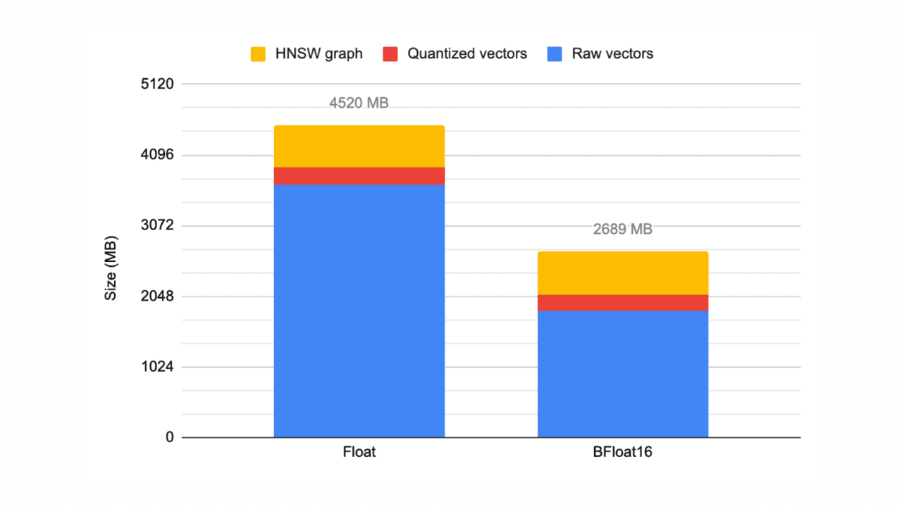
Elasticsearch 9.3 adds bfloat16 vector support
Exploring the new Elasticsearch element_type: bfloat16, which can halve your vector data storage.
February 10, 2026
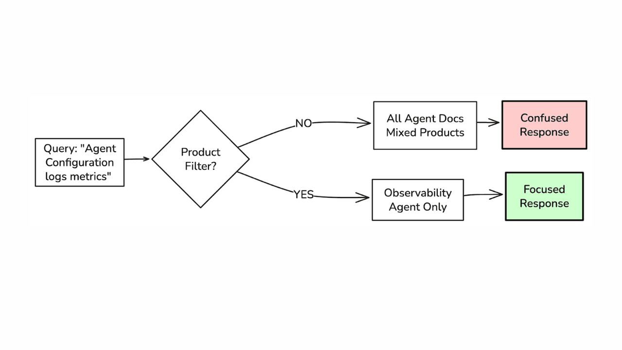
How to defend your RAG system from context poisoning
How context engineering techniques prevent context poisoning in LLM responses.
February 4, 2026
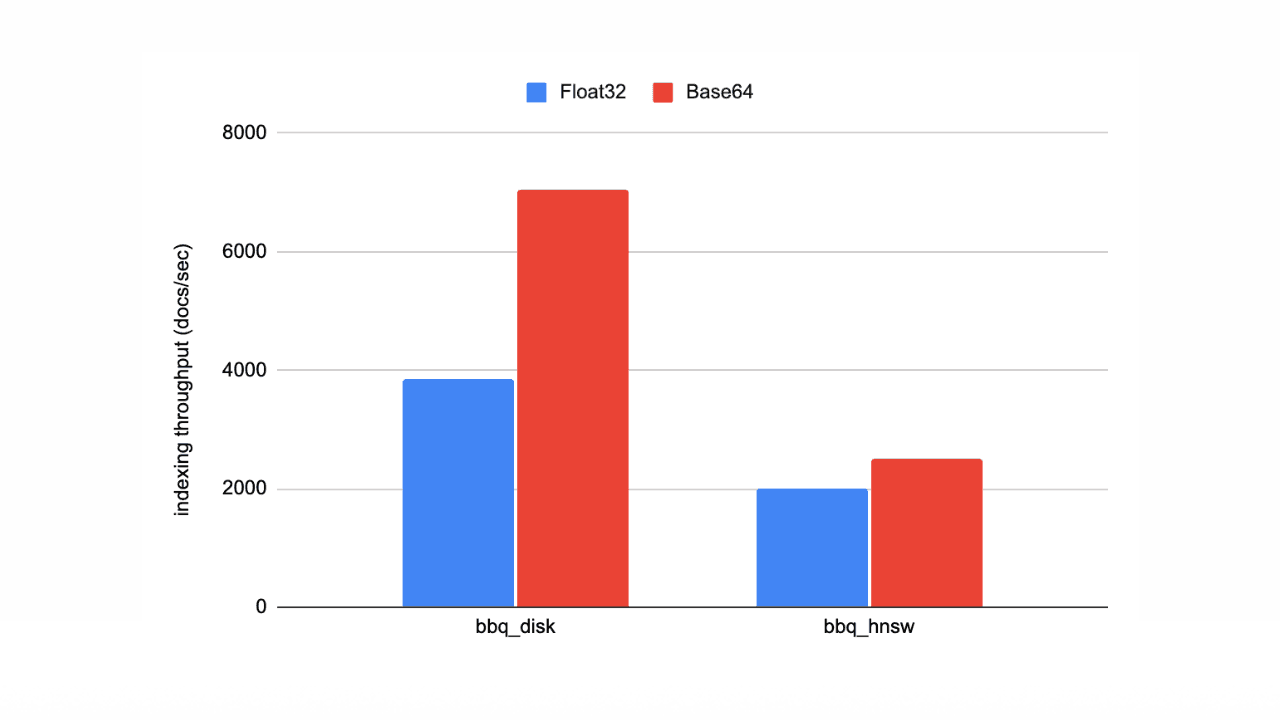
Speed up vector ingestion using Base64-encoded strings
Introducing Base64-encoded strings to speed up vector ingestion in Elasticsearch.

February 5, 2026
ES|QL dense vector search support
Using ES|QL for vector search on your dense_vector data.

January 28, 2026
Apache Lucene 2025 wrap-up
2025 was a stellar year for Apache Lucene; here are our highlights.