- Elasticsearch Guide: other versions:
- Getting Started
- Setup Elasticsearch
- Breaking changes
- Breaking changes in 5.0
- Search and Query DSL changes
- Mapping changes
- Percolator changes
- Suggester changes
- Index APIs changes
- Document API changes
- Settings changes
- Allocation changes
- HTTP changes
- REST API changes
- CAT API changes
- Java API changes
- Packaging
- Plugin changes
- Filesystem related changes
- Path to data on disk
- Aggregation changes
- Script related changes
- Breaking changes in 5.0
- API Conventions
- Document APIs
- Search APIs
- Aggregations
- Metrics Aggregations
- Avg Aggregation
- Cardinality Aggregation
- Extended Stats Aggregation
- Geo Bounds Aggregation
- Geo Centroid Aggregation
- Max Aggregation
- Min Aggregation
- Percentiles Aggregation
- Percentile Ranks Aggregation
- Scripted Metric Aggregation
- Stats Aggregation
- Sum Aggregation
- Top hits Aggregation
- Value Count Aggregation
- Bucket Aggregations
- Children Aggregation
- Date Histogram Aggregation
- Date Range Aggregation
- Diversified Sampler Aggregation
- Filter Aggregation
- Filters Aggregation
- Geo Distance Aggregation
- GeoHash grid Aggregation
- Global Aggregation
- Histogram Aggregation
- IP Range Aggregation
- Missing Aggregation
- Nested Aggregation
- Range Aggregation
- Reverse nested Aggregation
- Sampler Aggregation
- Significant Terms Aggregation
- Terms Aggregation
- Pipeline Aggregations
- Avg Bucket Aggregation
- Derivative Aggregation
- Max Bucket Aggregation
- Min Bucket Aggregation
- Sum Bucket Aggregation
- Stats Bucket Aggregation
- Extended Stats Bucket Aggregation
- Percentiles Bucket Aggregation
- Moving Average Aggregation
- Cumulative Sum Aggregation
- Bucket Script Aggregation
- Bucket Selector Aggregation
- Serial Differencing Aggregation
- Matrix Aggregations
- Caching heavy aggregations
- Returning only aggregation results
- Aggregation Metadata
- Metrics Aggregations
- Indices APIs
- Create Index
- Delete Index
- Get Index
- Indices Exists
- Open / Close Index API
- Shrink Index
- Rollover Index
- Put Mapping
- Get Mapping
- Get Field Mapping
- Types Exists
- Index Aliases
- Update Indices Settings
- Get Settings
- Analyze
- Index Templates
- Shadow replica indices
- Indices Stats
- Indices Segments
- Indices Recovery
- Indices Shard Stores
- Clear Cache
- Flush
- Refresh
- Force Merge
- cat APIs
- Cluster APIs
- Query DSL
- Mapping
- Analysis
- Anatomy of an analyzer
- Testing analyzers
- Analyzers
- Tokenizers
- Token Filters
- Standard Token Filter
- ASCII Folding Token Filter
- Length Token Filter
- Lowercase Token Filter
- Uppercase Token Filter
- NGram Token Filter
- Edge NGram Token Filter
- Porter Stem Token Filter
- Shingle Token Filter
- Stop Token Filter
- Word Delimiter Token Filter
- Stemmer Token Filter
- Stemmer Override Token Filter
- Keyword Marker Token Filter
- Keyword Repeat Token Filter
- KStem Token Filter
- Snowball Token Filter
- Phonetic Token Filter
- Synonym Token Filter
- Compound Word Token Filter
- Reverse Token Filter
- Elision Token Filter
- Truncate Token Filter
- Unique Token Filter
- Pattern Capture Token Filter
- Pattern Replace Token Filter
- Trim Token Filter
- Limit Token Count Token Filter
- Hunspell Token Filter
- Common Grams Token Filter
- Normalization Token Filter
- CJK Width Token Filter
- CJK Bigram Token Filter
- Delimited Payload Token Filter
- Keep Words Token Filter
- Keep Types Token Filter
- Classic Token Filter
- Apostrophe Token Filter
- Decimal Digit Token Filter
- Fingerprint Token Filter
- Minhash Token Filter
- Character Filters
- Modules
- Index Modules
- Ingest Node
- Pipeline Definition
- Ingest APIs
- Accessing Data in Pipelines
- Handling Failures in Pipelines
- Processors
- Append Processor
- Convert Processor
- Date Processor
- Date Index Name Processor
- Fail Processor
- Foreach Processor
- Grok Processor
- Gsub Processor
- Join Processor
- JSON Processor
- Lowercase Processor
- Remove Processor
- Rename Processor
- Script Processor
- Set Processor
- Split Processor
- Sort Processor
- Trim Processor
- Uppercase Processor
- Dot Expander Processor
- How To
- Testing
- Glossary of terms
- Release Notes
- 5.0.2 Release Notes
- 5.0.1 Release Notes
- 5.0.0 Combined Release Notes
- 5.0.0 GA Release Notes
- 5.0.0-rc1 Release Notes
- 5.0.0-beta1 Release Notes
- 5.0.0-alpha5 Release Notes
- 5.0.0-alpha4 Release Notes
- 5.0.0-alpha3 Release Notes
- 5.0.0-alpha2 Release Notes
- 5.0.0-alpha1 Release Notes
- 5.0.0-alpha1 Release Notes (Changes previously released in 2.x)
WARNING: Version 5.0 of Elasticsearch has passed its EOL date.
This documentation is no longer being maintained and may be removed. If you are running this version, we strongly advise you to upgrade. For the latest information, see the current release documentation.
Serial Differencing Aggregation
editSerial Differencing Aggregation
editThis functionality is in technical preview and may be changed or removed in a future release. Elastic will work to fix any issues, but features in technical preview are not subject to the support SLA of official GA features.
Serial differencing is a technique where values in a time series are subtracted from itself at different time lags or periods. For example, the datapoint f(x) = f(xt) - f(xt-n), where n is the period being used.
A period of 1 is equivalent to a derivative with no time normalization: it is simply the change from one point to the next. Single periods are useful for removing constant, linear trends.
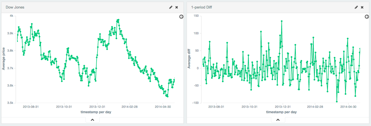
Single periods are also useful for transforming data into a stationary series. In this example, the Dow Jones is plotted over ~250 days. The raw data is not stationary, which would make it difficult to use with some techniques.
By calculating the first-difference, we de-trend the data (e.g. remove a constant, linear trend). We can see that the data becomes a stationary series (e.g. the first difference is randomly distributed around zero, and doesn’t seem to exhibit any pattern/behavior). The transformation reveals that the dataset is following a random-walk; the value is the previous value +/- a random amount. This insight allows selection of further tools for analysis.
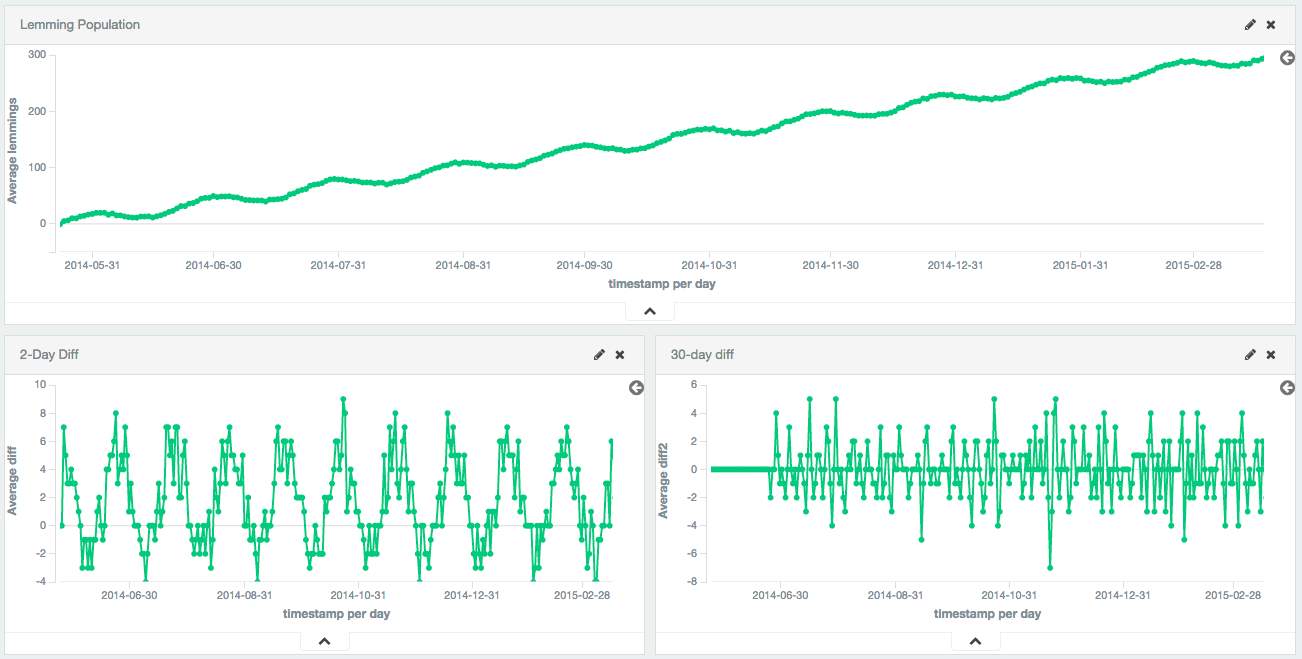
Larger periods can be used to remove seasonal / cyclic behavior. In this example, a population of lemmings was synthetically generated with a sine wave + constant linear trend + random noise. The sine wave has a period of 30 days.
The first-difference removes the constant trend, leaving just a sine wave. The 30th-difference is then applied to the first-difference to remove the cyclic behavior, leaving a stationary series which is amenable to other analysis.
Syntax
editA serial_diff aggregation looks like this in isolation:
{
    "serial_diff": {
        "buckets_path": "the_sum",
        "lag": "7"
    }
}
Table 13. serial_diff Parameters
| Parameter Name | Description | Required | Default Value |
|---|---|---|---|
|
Path to the metric of interest (see |
Required |
|
|
The historical bucket to subtract from the current value. E.g. a lag of 7 will subtract the current value from the value 7 buckets ago. Must be a positive, non-zero integer |
Optional |
|
|
Determines what should happen when a gap in the data is encountered. |
Optional |
|
|
Format to apply to the output value of this aggregation |
Optional |
|
serial_diff aggregations must be embedded inside of a histogram or date_histogram aggregation:
POST /_search
{
   "size": 0,
   "aggs": {
      "my_date_histo": {
         "date_histogram": {
            "field": "timestamp",
            "interval": "day"
         },
         "aggs": {
            "the_sum": {
               "sum": {
                  "field": "lemmings"
               }
            },
            "thirtieth_difference": {
               "serial_diff": {
                  "buckets_path": "the_sum",
                  "lag" : 30
               }
            }
         }
      }
   }
}
|
A |
|
|
A |
|
|
Finally, we specify a |
Serial differences are built by first specifying a histogram or date_histogram over a field. You can then optionally
add normal metrics, such as a sum, inside of that histogram. Finally, the serial_diff is embedded inside the histogram.
The buckets_path parameter is then used to "point" at one of the sibling metrics inside of the histogram (see
buckets_path Syntax for a description of the syntax for buckets_path.
On this page