Anomaly detection population jobs: Spotify Wrapped, part 3

In the first part, we talked about how to get your Spotify Wrapped data and how to visualize it. In the second part, we talked about how to process the data and how to visualize it. In this third part, we will talk about how to detect anomalies in your Spotify Wrapped data.

What is an anomaly detection job?

An anomaly detection job in Elastic tries to find unusual patterns in your data. It uses machine learning to learn the normal behavior of your data and then tries to find data points that do not fit this normal behavior. This can be useful for finding unusual patterns in your data, like a sudden increase in the number of songs you listened to or a sudden change in the average duration of the songs you listened to.

There are many different types of anomaly detection jobs:

Single metric
Multi-metric
Population
Categorization
Rare
Geo
Advanced

Now, we will take a look at a few of those.

Population job

A population job is a type of anomaly detection job that tries to find unusual patterns in the distribution of your data. The distribution is defined by the population. Let's create that job together!

1. Go to the Machine Learning app in Kibana.

2. Click on "Create job."

3. Select the Spotify-History data view (if you do not have that one yet, don't forget to import the dashboard and data view from here).

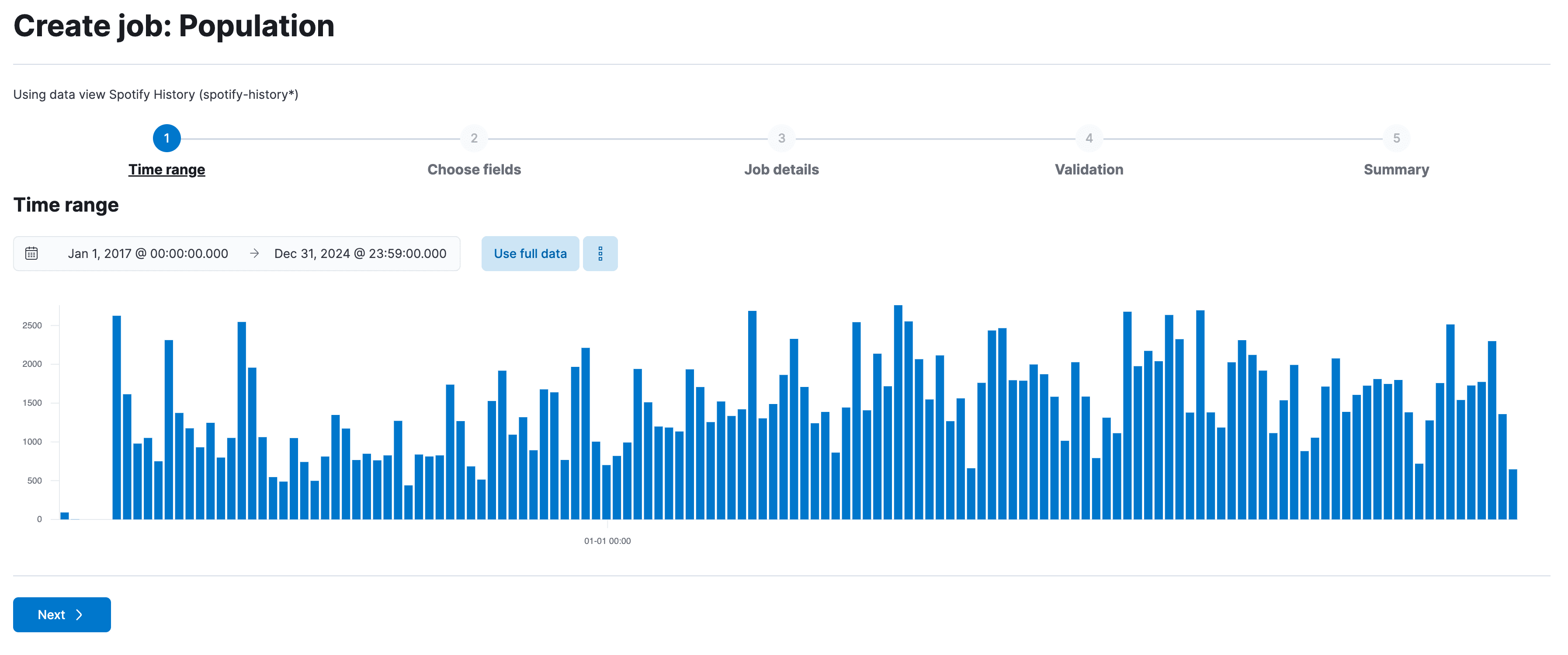
4. Select Population.

5. Select a proper timeframe, for me that is 1st January 2017 and 31st December 2024.

6. Select the field you want to define your population on. Let's use artist.

7. For the Add Metric, we want to use sum(listened_to_ms). This will sum up the total time you listened to a specific artist.

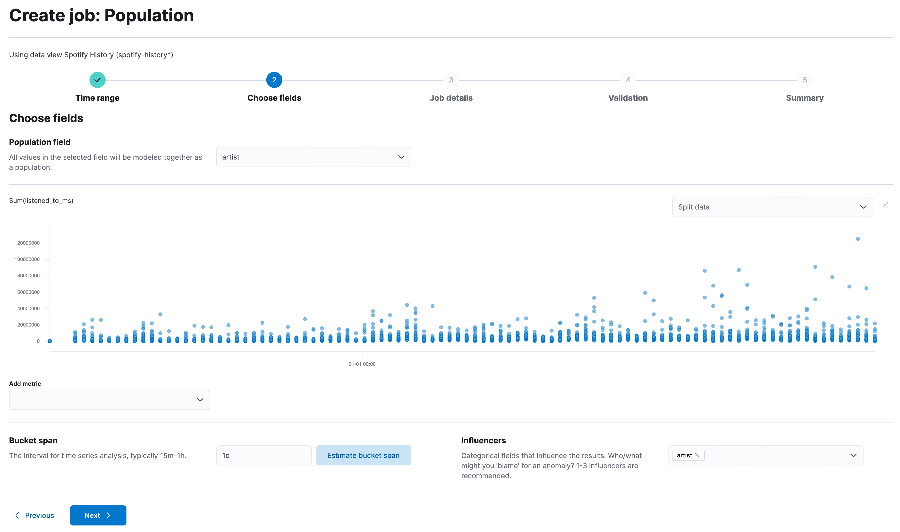
8. In the right bottom for influencers, add the title. This will give us more information when an anomaly occurs.

9. Bucket Span so that is a big point to discuss. In my case, I do not think there is any sense in looking at something different than a daily pattern. You might even want to check out weekly patterns. It really depends on a lot of factors. Going lower than 1 day could be a bit too fine, and therefore, you'll get not optimal results.

10. Click on next, give it a valid name and click next until it says create job. Ensure that the toggle for Start immediately is turned on. Click create job. It will start immediately and probably look like this:

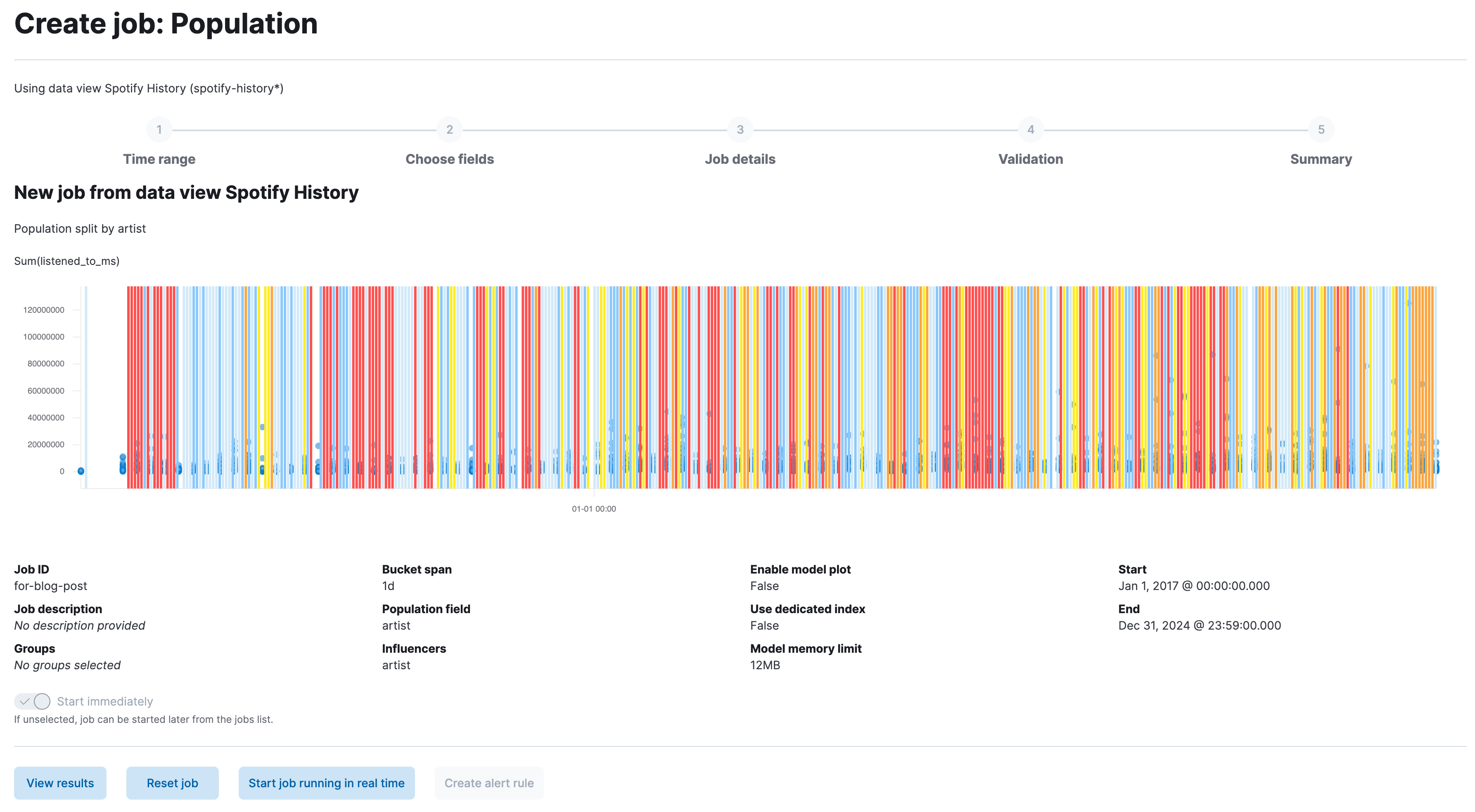
Perfect, let's dive into the details. Click View Results—this page will be very interesting for our analysis

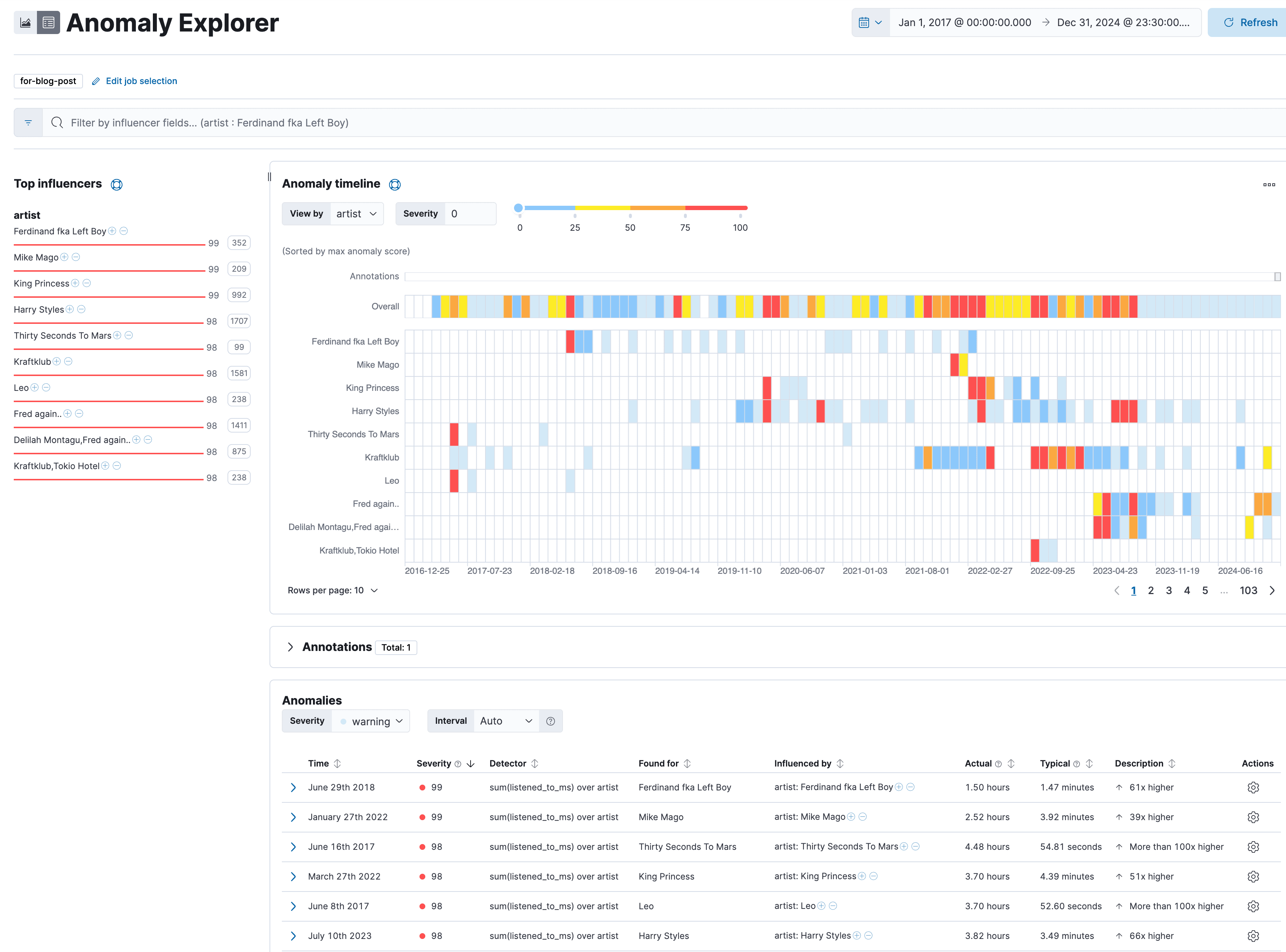
Interpreting that is simple. Everything red is a higher scoring anomaly and everything blue or lighter shaded is less high. We immediately spot that on the right-hand side, the band Kraftklub has some bars in red, orange, red, and shading out to blue.

When focusing on Kraftklub by doing artist: Kraftklub in the search bar on top, it immediately tells me: September 30th, 2022 Actual 3.15 hours instead of 3.75 minutes. For me, that means that I regularly listen to roughly one song of Kraftklub per day, on this day I listened to over 3 hours of Kraftklub. That is clearly an anomaly. What could have triggered such a listening behavior? The concert was a bit far off, it was on the 19th of November, 2022. Maybe a new album that came out?

We can actually spot that by clicking on the anomaly and selecting the View in Discover from the dropdown.

Once we are in Discover, we can do additional visualizations and breakdowns to investigate this further. We will pull up the title, album and spotify_metadata.album.release_date to see if a new album came out on that day. We can immediately see that on 22nd September 2022, the album KARGO was released. 8 days later, it appears that I took an interest and started listening to it.

What else can we find? Maybe something seasonal? Let's zoom into Fred Again.. which I listen to a lot (as you can tell from blog number two). There are roughly 10 days back to back as an anomaly. on average, I listened roughly an hour per day to Fred Again.

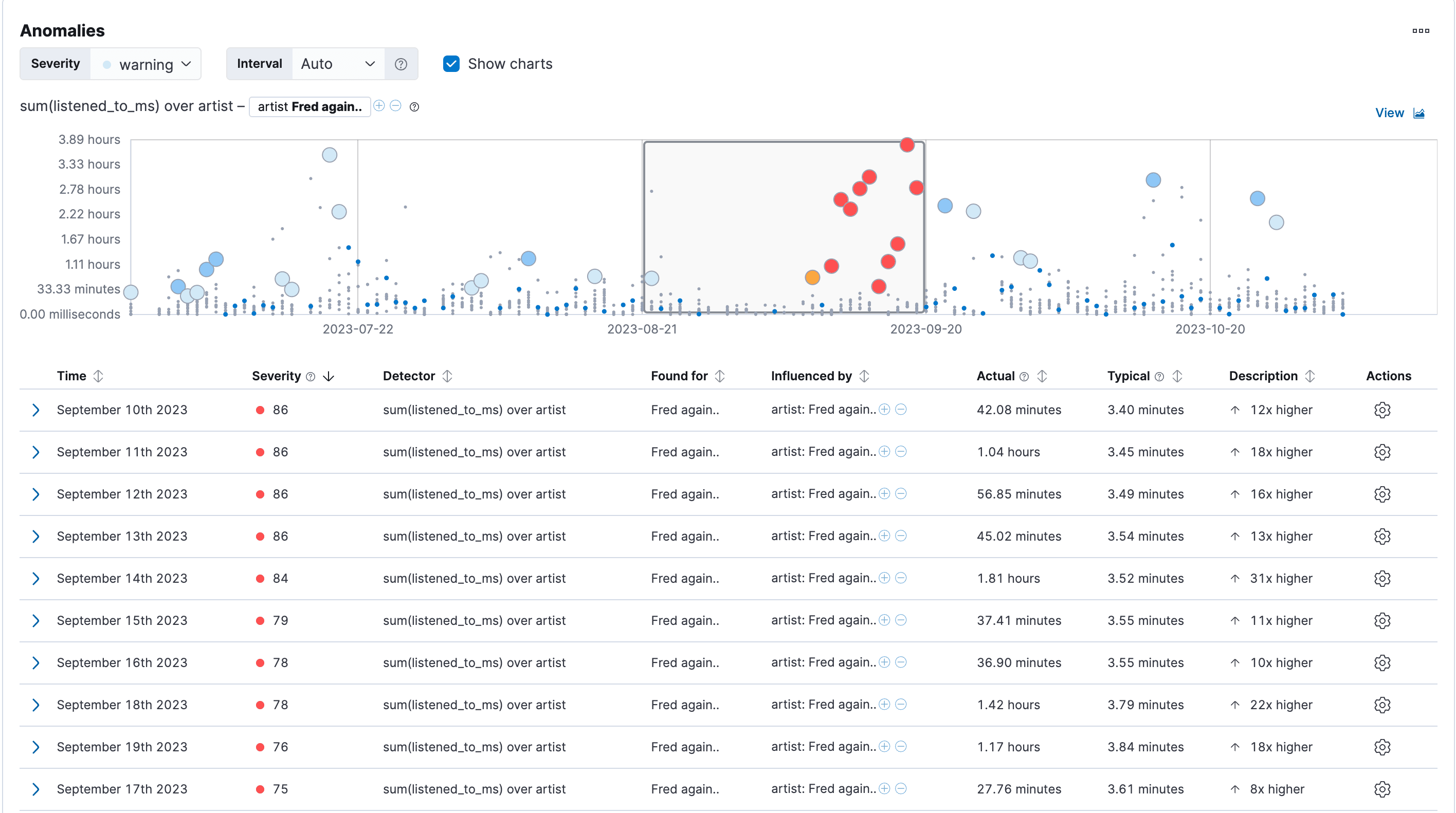
I know that Fred Again.. probably didn't release an album during that time. ES|QL will help us in figuring out more details. When switching to ES|QL, the time picker value will be kept, but any filters in the search bar will be removed. The first thing we need to do is to add that back.

FROM spotify-history
| WHERE artist=="Fred again.."

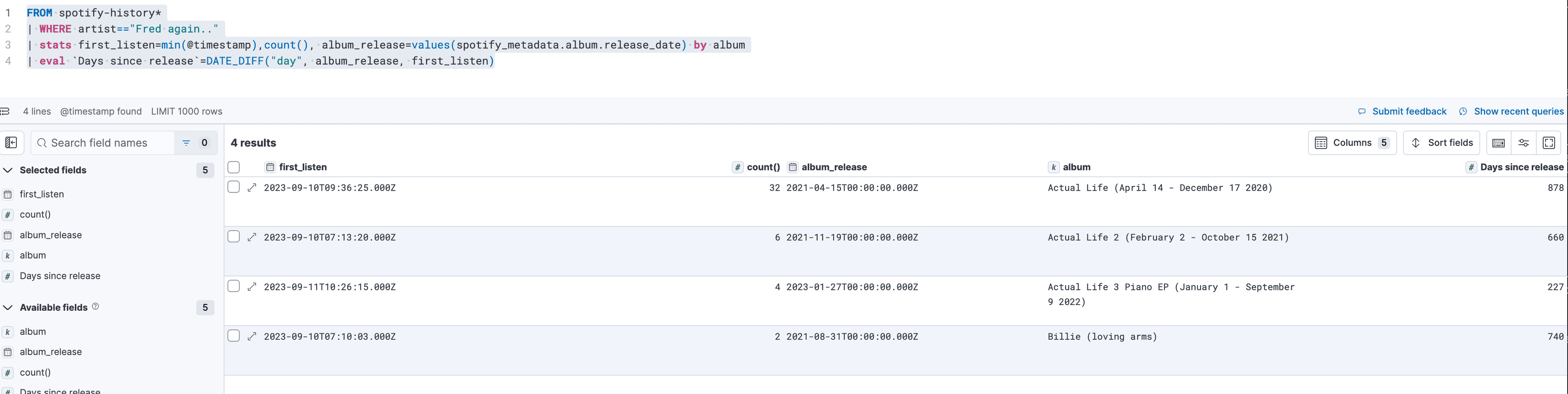
The next thing I want to know is how many albums I listened to and whether any were released near those days.

FROM spotify-history
| WHERE artist=="Fred again.."
| stats count(), values(spotify_metadata.album.release_date) by album

We perform a simple count to get the count of records. The values allow us to retrieve the value of the document and not perform any aggregation on it, and we split those up by the album name. I cannot spot any release date near the anomaly days. My "head date math" is not always on point, so let's add a difference in days from the release date to the first listen date (during this anomaly) as it is quite clear that an album release did not trigger this anomaly.

Single metric

A single metric job is a type of anomaly detection job that tries to find unusual patterns in a single metric. The metric is defined by the field you select. So, what could be an interesting single metric? Let's use the listened_to_pct. This tells us how much of a song I complete before I skip to the next one. This is quite intriguing—let’s see if there are certain days when I skip more than others.

1. Go to the Machine Learning app in Kibana.

2. Click on "Create job."

3. Select the Spotify-History data view.

4. Select Single Metric.

5. Select a proper timeframe, for me that is from 1st January 2017 to 31st December 2024.

Now it gets tricky, do we use mean(), high_mean(), low_mean()? Well, it depends on what we want to anomaly on. Mean will give you anomalies for low values such as 0, as well for high. High mean on the other hand is more on the high side, meaning that if the listening completion drops to 0 for a couple of days, it won't trigger an anomaly. Mean and low mean would. High mean is often useful when you want to detect spikes in your data. You don't want an anomaly if your service that is processing data is fast, you don't care if it finishes in 1 ms. But If it takes 10 ms, you want an anomaly.

In this case, I guess we should try mean() and see where it takes us.

6. Don't forget to set the bucket to 1 day.

7. Click on next, give it a valid name and click next until it says create job. Ensure that the toggle for Start immediately is turned on. Click create job. It will start immedaitely.

Here are the results:

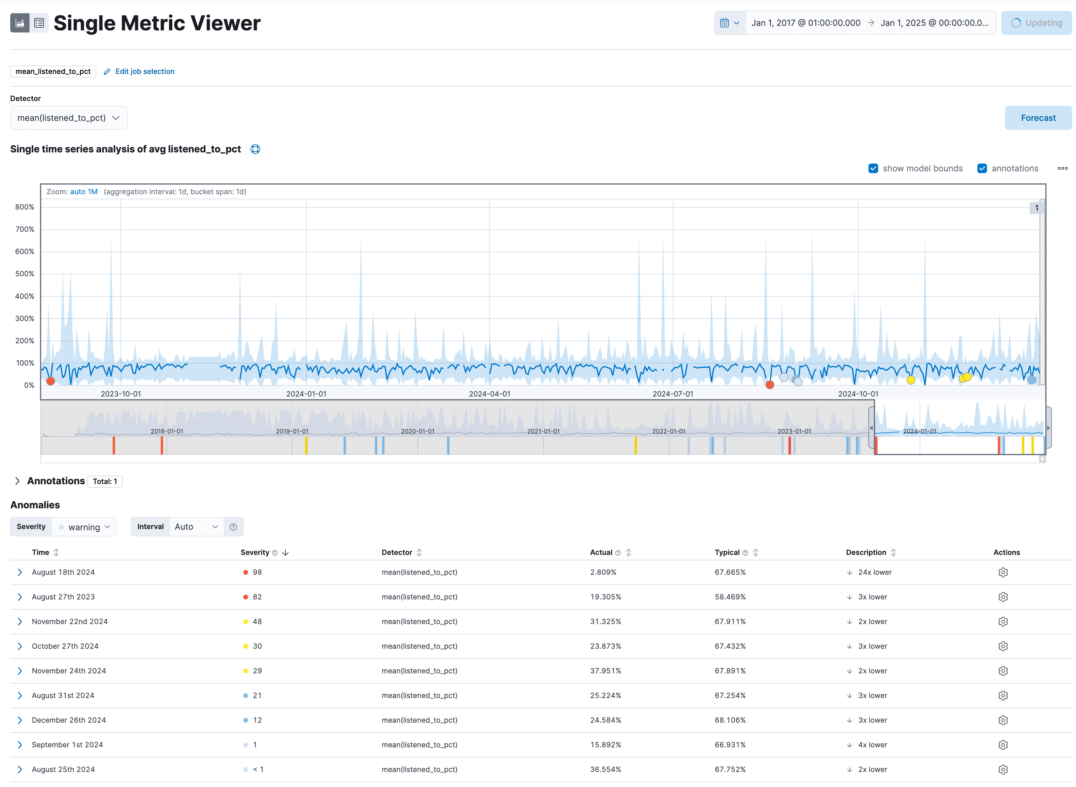
It's fascinating to see that on 18th August 2024, I only listened to songs for ~3% of their total duration on average. Usually, I listen to nearly 70% of the song before pressing the next button. All in all, I would say that mean() is a good choice for this metric.

Multi metric

Now, I want to figure out if I have a single song that spikes within an artist. To do that, we can leverage a multi metric job.

1. Go to the Machine Learning app in Kibana.

2. Click on "Create job."

3. Select the Spotify-History data view.

4. Select Multi Metric.

5. Select a proper timeframe, for me that is from 1st January 2017 to 31st December 2024.

6. Select the distinct count(title) and split by artist, add artist, title, album to the influencers.

7. Don't forget the bucket span to 1d.

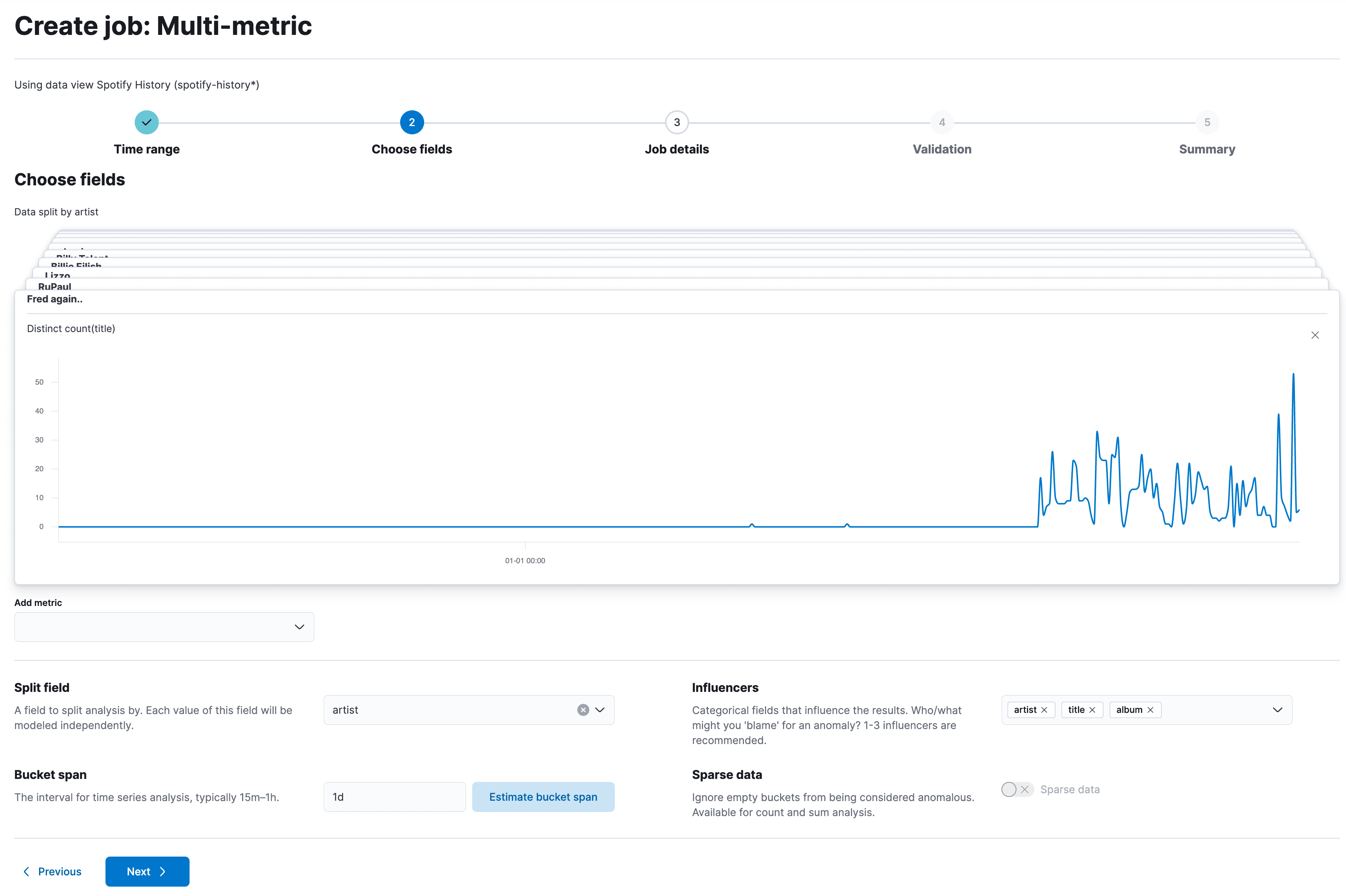
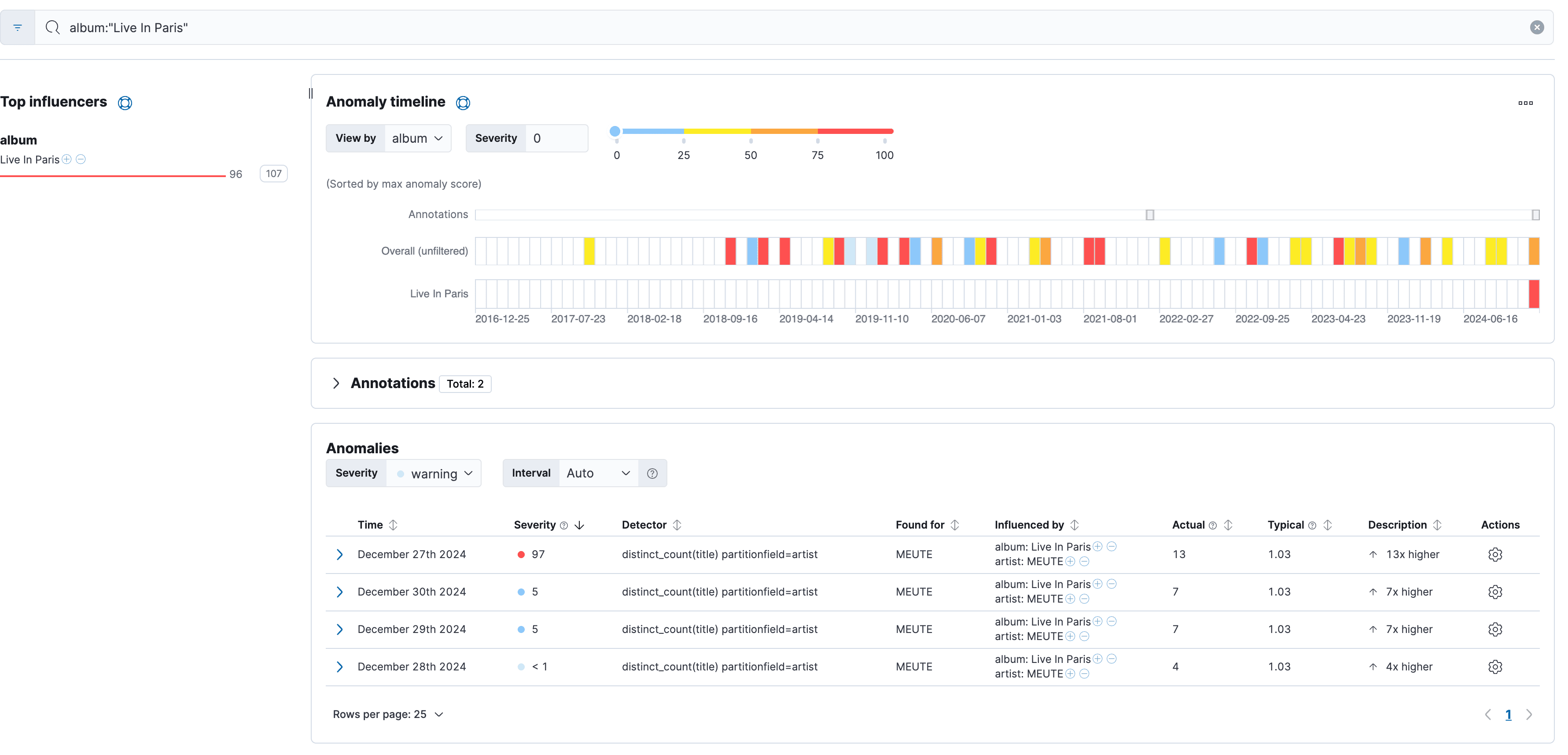
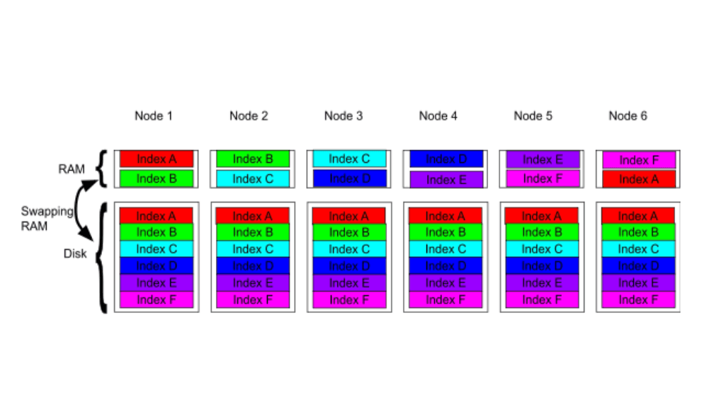
It might give you a warning about high memory usage because instead of modeling everything in one large model, it now creates a single model for each artist. This can be quite memory intensive, so be careful. Go into the same anomaly detection table view and pick any album at random. I chose Live in Paris from Meute. At first glance, that's super interesting and it shows how accurate anomaly detection can be.

I have the song You & Me from the album Live in Paris in my liked songs as well as roughly 10 other songs from different albums. I actively listened to the Live in Paris album on the 27th, 28th, 29th and 30th of December 2024.

Conclusion

In this blog, we dived into the rabbit hole of anomaly detection and what that can entail. It might be daunting at first, but it's not that complicated once you get a hang of it and it can also provide really good and quick insights.

The release and timing of any features or functionality described in this post remain at Elastic's sole discretion. Any features or functionality not currently available may not be delivered on time or at all.

In this blog post, we may have used or referred to third party generative AI tools, which are owned and operated by their respective owners. Elastic does not have any control over the third party tools and we have no responsibility or liability for their content, operation or use, nor for any loss or damage that may arise from your use of such tools. Please exercise caution when using AI tools with personal, sensitive or confidential information. Any data you submit may be used for AI training or other purposes. There is no guarantee that information you provide will be kept secure or confidential. You should familiarize yourself with the privacy practices and terms of use of any generative AI tools prior to use.

Elastic, Elasticsearch, ESRE, Elasticsearch Relevance Engine and associated marks are trademarks, logos or registered trademarks of Elasticsearch N.V. in the United States and other countries. All other company and product names are trademarks, logos or registered trademarks of their respective owners.

Want to get Elastic certified? Find out when the next Elasticsearch Engineer training is running!

Elasticsearch is packed with new features to help you build the best search solutions for your use case. Dive into our sample notebooks to learn more, start a free cloud trial, or try Elastic on your local machine now.

Report an issue