Elasticsearch is packed with new features to help you build the best search solutions for your use case. Learn how to put them into action in our hands-on webinar on building a modern Search AI experience. You can also start a free cloud trial or try Elastic on your local machine now.
In our previous blog on ColPali, we explored how to create visual search applications with Elasticsearch. We primarily focused on the value that models such as ColPali bring to our applications, but they come with performance drawbacks compared to vector search with bi-encoders such as E5.
Building on the examples from part 1, this blog explores how to use different techniques and Elasticsearch's powerful vector search toolkit in order to make late interaction vectors ready for large-scale production workloads.
The full code examples can be found on GitHub.
Challenges of late interaction models
ColPali creates over 1000 vectors per page for the documents in our index.
This results in two challenges when working with late interaction vectors:
- Disk space: Saving all these vectors on disks will incur a serious amount of storage usage, which will be expensive at scale.
- Computation: When ranking our documents with the
maxSimDotProduct()comparison, we need to compare all of these vectors for each of our documents with the N vectors of our query.
Let’s look at some techniques for addressing these issues.
Techniques to optimize late interaction models
Bit vectors
In order to reduce disk space, we can compress the images into bit vectors. We can use a simple Python function to transform our multi-vectors into bit vectors:
The function's core concept is straightforward: values above 0 become 1, and values below 0 become 0. This results in an array of 0s and 1s, which we then transform into a hexadecimal string representing our bit vector.
For our index mapping, we set the element_type parameter to bit:
After having written all of our new bit vectors to our index, we can rank our bit vectors using the following code:

Trading off a bit of accuracy, this allows us to use hamming distance (maxSimInvHamming(...)), which is able to leverage optimizations such as bit-masks, SIMD, etc. Learn more about bit vectors and hamming distance in our blog.
Alternatively, we can not convert our query vector to bit vectors and search with the full-fidelity late interaction vector:

This will compare our vectors using an asymmetric similarity function.
Let’s think about a regular hamming distance between two bit vectors. Suppose we have a document vector D:

And a query vector Q:

Simple binary quantization will transform vectors D into 10101101 and Q into 11111011. To find the hamming distance, we need direct bit math—it's extremely fast. In this case, the hamming distance is 01010110, which has a bit count of 4. So, scoring then becomes the inverse of that hamming distance. Remember, more similar vectors have a SMALLER hamming distance, so inverting it allows for more similar vectors to be scored higher. Specifically here, the score would be 1/4 = 0.25.
However, note how we lose the magnitude of each dimension. A 1 is a 1. So, for Q, the difference between 0.01 and 0.79 disappears. Since we are simply quantizing according to >0, we can do a small trick where the Q vector isn’t quantized. This doesn’t allow for the extremely fast bitwise math, but it does keep the storage cost low as D is still quantized.

In short, this retains the information provided in Q, thus increasing the distance estimation quality and keeping the storage low.
Using bit vectors allows us to save significantly on disk space and computational load at query time. But there is more that we can do.
Average vectors
To scale our search across hundreds of thousands of documents, even the performance benefits that bit vectors give us will not be enough. In order to scale to these types of workloads, we will want to leverage Elasticsearch’s HNSW index structure for vector search.
ColPali generates around a thousand vectors per document, which is too many to add to our HNSW graph. Therefore, we need to reduce the number of vectors. To do this, we can create a single representation of the document's meaning by taking the average of all the document vectors produced by ColPali when we embed our image.

We simply take the average vector over all late interaction vectors.
As of now, this is not possible within Elastic itself, and we will need to preprocess the vectors before ingesting them in Elasticsearch.
We can do this with Logstash or Ingest pipelines, but here we will use a simple Python function:
We are also normalizing the vector so that we can use the dot product similarity.
After transforming all of our ColPali vectors to average vectors, we can index them into our dense_vector field:
We have to consider that this will increase total disk usage since we are saving more information along with our late interaction vectors. Additionally, we will use extra RAM to hold the HNSW graph, allowing us to scale the search over billions of vectors. To reduce the usage of RAM, we can make use of our popular BBQ feature. In turn, we get fast search results over massive data sets that would otherwise not be possible.
Now, we simply search with the knn query to find our most relevant documents.

The previously best match has unfortunately fallen to rank 3.
To fix this problem, we can do a multi-stage retrieval. In our first stage, we are using the knn query to search for the best candidates for our query over millions of documents. In the second stage, we are only reranking the top k (here: 10) with the higher fidelity of the ColPali late interaction vectors.

Here, we are using the in 8.18 introduced rescore retriever to rerank our results. After rescoring we see that our best match is again in first position.
Note: In a production application, we can use a much higher k than 10 as the max sim function is still comparatively performant.
Token pooling
Token pooling reduces the sequence length of multi-vector embeddings by pooling redundant information, such as white background patches. This technique decreases the number of embeddings while preserving most of the page's signal.

We are clustering semantically similar vectors to achieve less vectors overall.
Token pooling works by grouping similar token embeddings within a document into clusters using a clustering algorithm. Then, the mean of the vectors in each cluster is calculated to create a single, aggregated representation. This aggregated vector replaces the original tokens in the group, reducing the total number of vectors without significant loss of document signal.
The ColPali paper proposes an initial pool factor value of 3 for most datasets, which maintains 97.8% of the original performance while reducing the total number of vectors by 66.7%.

Source: https://arxiv.org/pdf/2407.01449
But we need to be careful: The "Shift" dataset, which contains very dense, text-heavy documents with little white space, declines rapidly in performance as pool factors increase.
To create the pooled vectors, we can use the colpali_engine library:
We now have a vector that was reduced by about 66.7% in its dimensions. We index it as usual and we are able to search on it with our maxSimDotProduct() function.

We are able to get good search results at the expense of some slight accuracy in the results.
Hint: With a higher pool_factor (100-200), you can also have a middle ground between the average vector solution and the one we discussed here. With around 5-10 vectors per document, it becomes viable to index them in a nested field to leverage the HNSW index.
Coss-encoder vs. late-interaction vs. bi-encoder
With what we have learned so far, where does this place late interaction models, such as ColPali or ColBERT, when we compare them to other AI retrieval techniques?
While the max sim function is cheaper compared to cross-encoders, it still requires many more comparisons and computation than vector search with bi-encoders, where we are just comparing two vectors for each query-document pair.

Because of this, our recommendation for late-interaction models is to generally only use them for reranking the top k search results. We also capture this in the name of the field type: rank_vectors.
But what about the cross encoder? Are late interaction models better because they are cheaper to execute at query time? As is often the case, the answer is: it depends. Cross encoders generally produce higher quality results, but they require a lot of compute because the query document pairs need to do a full pass through the transformer model. They also benefit from the fact that they do not require any indexing of vectors and can operate in a stateless manner. This results in:
- Less disk space used
- A simpler system
- Higher quality of search results
- Higher latency, and therefore not being able to rerank as deep
On the other hand, late Interaction models can offload some of this computation at index them, making the query cheaper. The price we pay is having to index the vectors, which makes our indexing pipelines more complex and also requires more disk space to save these vectors.
Specifically in the case of ColPali, the analysis of information from images is very expensive as they contain a lot of data. In this case, the tradeoff shifts in favor of using a late interaction model such as ColPali because evaluating this information at query time would be too resource-intensive/slow.
For a late interaction model such as ColBERT, which works on text data like most cross-encoders (e.g., elastic-rerank-v1), the decision might lean more toward using the cross-encoder to benefit from the disk savings and simplicity.
We encourage you to weigh those pros and cons for your use case and experiment with the different tools that Elasticsearch provides you to build the best search applications.
Conclusion
In this blog, we explored various techniques to optimize late interaction models like ColPali for large-scale vector search in Elasticsearch. While late interaction models provide a strong balance between retrieval efficiency and ranking quality, they also introduce challenges related to storage and computation.
To address these challenges, we looked at:
- Bit vectors to significantly reduce disk space while leveraging efficient similarity computations like hamming distance or asymmetric max similarity.
- Average vectors to compress multiple embeddings into a single dense representation, enabling efficient retrieval with HNSW indexing.
- Token pooling to intelligently merge redundant embeddings while maintaining semantic integrity, reducing computational overhead at query time.
Elasticsearch provides a powerful toolkit to customize and optimize search applications based on your needs. Whether you prioritize retrieval speed, ranking quality, or storage efficiency, these tools and techniques allow you to balance performance and quality as you need for your real-world applications.
Related Content

February 20, 2026
Ensuring semantic precision with minimum score
Improve semantic precision by employing minimum score thresholds. The article includes concrete examples for semantic and hybrid search.
February 17, 2026
An open‑source Hebrew analyzer for Elasticsearch lemmatization
An open-source Elasticsearch 9.x analyzer plugin that improves Hebrew search by lemmatizing tokens in the analysis chain for better recall across Hebrew morphology.
February 16, 2026
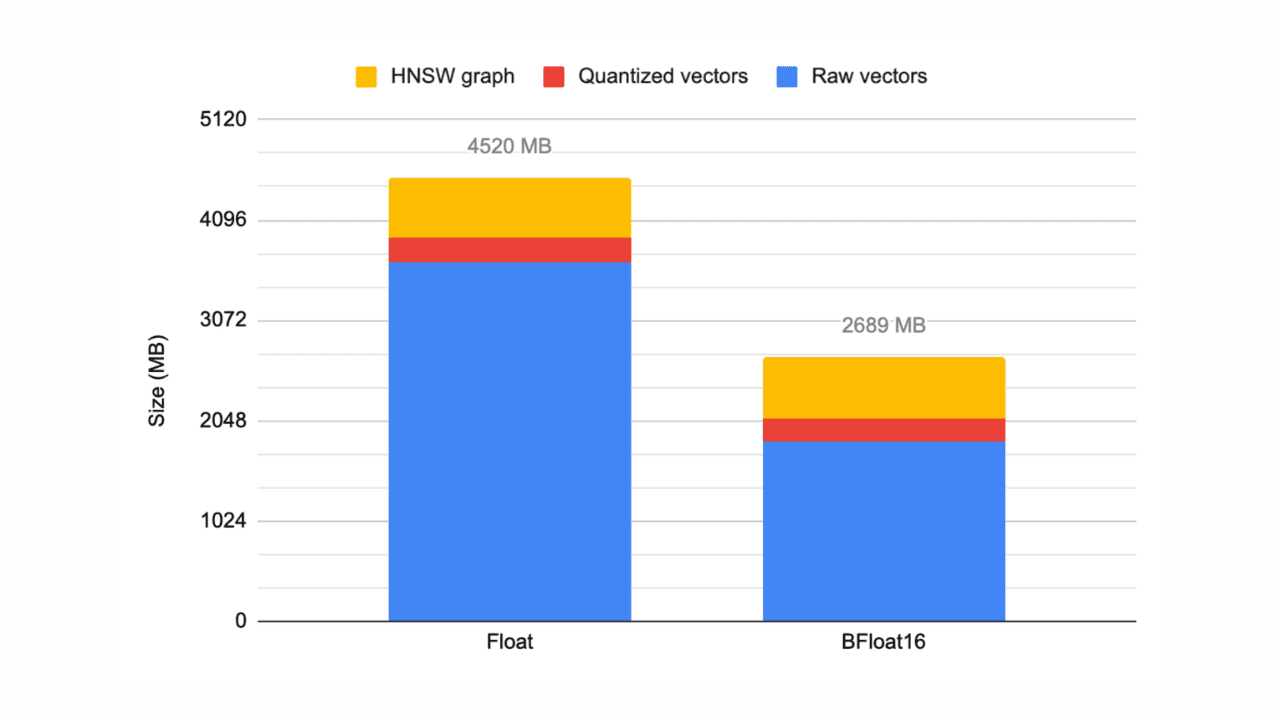
Elasticsearch 9.3 adds bfloat16 vector support
Exploring the new Elasticsearch element_type: bfloat16, which can halve your vector data storage.
February 10, 2026
How to defend your RAG system from context poisoning
How context engineering techniques prevent context poisoning in LLM responses.
January 30, 2026
Query rewriting strategies for LLMs and search engines to improve results
Exploring query rewriting strategies and explaining how to use the LLM's output to boost the original query's results and maximize search relevance and recall.