Timelion Tutorial – From Zero to Hero

This tutorial was crossposted on Tim's private blog.

Timelion is a visualization tool for time series in Kibana. Time series visualizations are visualizations, that analyze data in time order. Timelion can be used to draw two dimensional graphs, with the time drawn on the x-axis.

What's the advantage over just using plain bar or line visualizations? Timelion takes a different approach. Instead of using a visual editor to create charts, you define a graph by chaining functions together, using a timelion specific syntax. This syntax enables some features, that classical point series charts don't offer - like drawing data from different indices or data sources into one graph.

This tutorial will first give a short introduction to the timelion UI in Kibana and will afterwards explain the timelion syntax and show several use cases, that you couldn't or still cannot do with classical Kibana visualizations.

The user interface

You can access timelion from the main navigation on the left of the page.

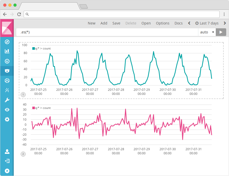
You can have multiple graphs on a timelion sheet. To add a new graph to the sheet use the Add link in the top menu bar. New will create a completely new sheet.

The input box on top of the window shows the expression for the currently selected graph. Click on a graph to select it for editing. All expressions you will see throughout this tutorial will be inserted into that textbox.

Using the Save button in the menu, you can either store the whole timelion sheet with all its graphs or store the currently focused graph as a visualization, that you can place on any dashboard.

The date range of the currently shown data can be influenced by the well-known date picker on the top right of the page. To set the scale of the x-axis, the selectbox beside the expression input is used. By default it's set to "auto" which will automatically determine what a good scale would be depending on the selected time range. If you want to force e.g. one data point per day, you can set this to 1d.

Timelion expressions

The simplest expression - that will also automatically be used for new graphs is the following:

.es(*)

Timelion functions always start with a dot, followed by the function name, followed by parentheses containing all the parameters to the function (in this case just the asterisk).

The .es (or .elasticsearch if you are a fan of typing long words) function gathers data from Elasticsearch and draws it over time.

If you don't specify an index in the expression (we will see in a moment how you're able to do this) all indexes of your Elasticsearch will be queried for data. You can change this default in the Advanced Settings of Kibana by modifying the timelion:es.default_index setting.

By default the .es function will just count the number of documents, resulting in a graph showing the amount of documents over time.

If you are entering that simple expression and only get a flat line, even though you selected a date range, which contains data: most likely your data doesn't use @timestamp as the name for the main time field. You can either change the default name via the timelion:es.timefield setting in Advanced Settings, or use the timefield parameter in the .es function to set it for an individual series. You will see how to set parameters in the next section.

Function parameters

Functions can have multiple parameters, and so does the .es function. Each parameter has a name, that you can use inside the parentheses to set its value.

The parameters also have an order, which is shown by the autocompletion or the documentation (using the Docs button in the top menu).

If you don't specify the parameter name, timelion assigns the values to the parameters in the order, they are listed in the documentation.

The fist parameter of the .es function is the parameter q (for query), which is a Query String used to filter the data for this series. You can also explicitly reference this parameter by its name, and I would always recommend doing so as soon as you are passing more than one parameter to the function. The following two expressions are thus equivalent:

.es(*)
.es(q=*)

Multiple parameters are separated by comma. The .es function has another parameter called index, that can be used to specify an index pattern for this series, so the query won't be executed again all indexes (or whatever you changed the above mentioned setting to).

.es(q=*, index=logstash-*)

If the value of your parameter contains spaces or commas you have to put the value in single or double quotes. You can omit these quotes otherwise.

.es(q='some query', index=logstash-*)

Chaining functions

A lot of the timelion functions are used to modify a series of data. You apply these by chaining the functions in the expression. The .label function is such a function. You can use it to change the label of a series:

.es(q=country:de).label(Germany)

You can also chain multiple expressions, as we will see later in this tutorial.

Multiple series

One of the advantages of using timelion is the ability to add multiple time series to one chart. Multiple series must simply be separated by a comma in the expression:

.es(q=de), .es(q=us)

You can also chain functions on each series now, e.g. for specifying labels:

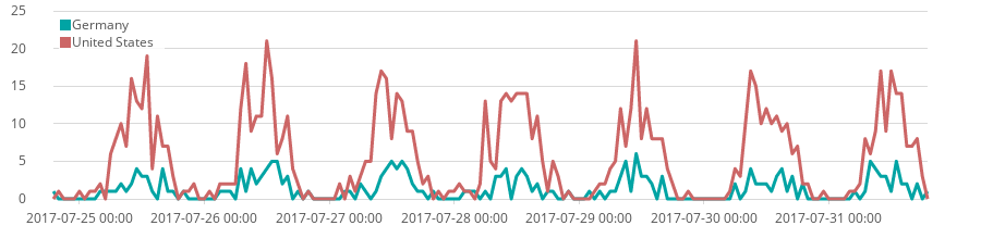
.es(q=de).label(Germany), .es(q=us).label('United States')

Now we covered the basics on how to work with timelion, so we can jump to a more in depth explanation of several functions and what you can do with them.

Timelion functions

To demonstrate the functions we will use some sample data, which contains access logs from a web server. The sample data was created using makelogs which you can use to create your own sample data.

Data source functions

Data source functions can be used to load data into the graph. We've already seen the .es data function, that loads data from Elasticsearch. Timelion offers some more sources to load data from, which we will explain in this section.

Elasticsearch

Before we have a look at the other data source functions, we should first look at the .es function again. It provides some more functionality, that we haven't seen yet.

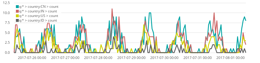
Since it is a common use case to split lines by the value of a specific field (what you can do with a terms aggregation in a regular visualization), the .es function has a parameter named split for that.

The value of the split parameter must be a fieldname, followed by a colon, followed by a numeric value, on how many of the top values should get a line. The following expression, shows the traffic of the top 4 countries (the country code is stored in the geo.dest field) in our sample data:

.es(split=country:4)

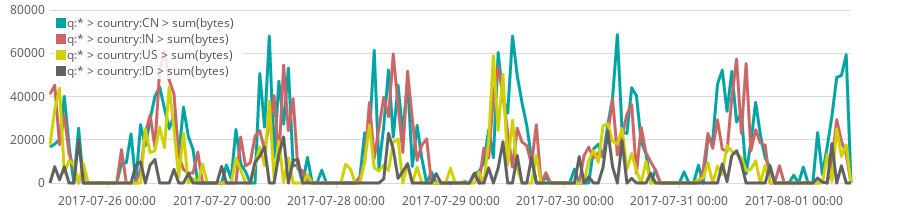
The metric parameter is used to control the calculation of the y-value. By default the .es function will put the count of documents on the y-axis. You can use the metric parameter to specify another metrics aggregation, that should be used to calculate the value at a specific time. The value must be the name of a single value metrics aggregation, followed by a colon, followed by the field name to calculate that aggregation on.

Valid names for the aggregation are e.g. avg to calculate the average value of a field, sum for the sum, cardinality to get the amount of unique values in a field, min and max to retrieve the minimum or maximum value of a field.

If we want to modify the above expression to display the top 4 countries by how many bytes has been transferes in that country (to see what countries are responsible for my bandwidth), you can use the metric parameter as follows:

.es(split=country:4, metric=sum:bytes)

You can also use multiple split parameters to create subbuckets (as in visualizations) and multiple metric parameters to draw multiple values per time point.

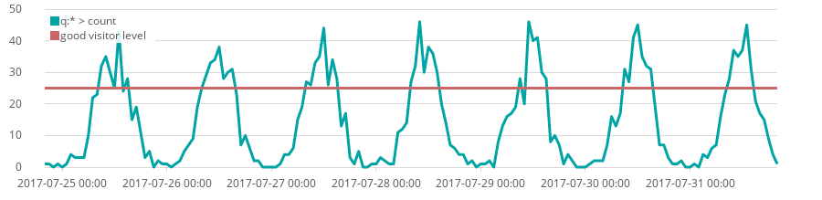
static/value

.static (or the alias .value) will just draw a plain horizontal line at the given value. This can be useful to draw a visual threshold to a graph. You can also use the parameter label to directly label the series:

.es(), .static(25, label='good visitor level')

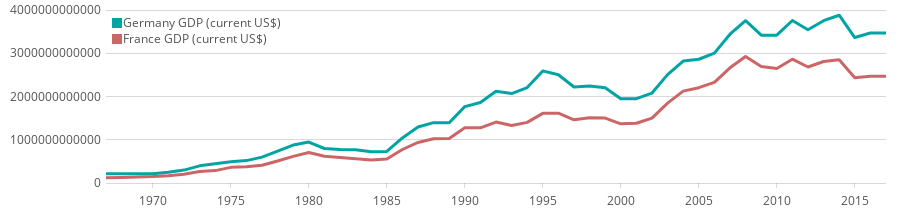
World Bank

Timelion offers functions to load data directly from World Bank, which provides a lot of statistical data from around the world, e.g. population, GDP, and many more.

To pull in data from World Bank into your graph, you can use the .wbi (or long .worldbank_indicators) function. It accepts two parameters: country and indicator.

country can be the ISO code of a specific country or if not specified data for the whole world will be loaded. indicator must be a valid World Bank indicator. You can find a list of all indicators on their data portal. If you click on an indicator, you can see the actual indicator code you need to specify in the URL, e.g. it's NY.GDP.MKTP.CD for the GDP of a country or SP.POP.0014.TO.ZS for the population ages 0 to 14 in percentage. If you don't specify an indicator the population is loaded.

To visualize the GDP of France and Germany, you could use the following expression:

.wbi(country=de, indicator=NY.GDP.MKTP.CD), .wbi(country=fr, indicator=NY.GDP.MKTP.CD)

If you need to manipulate the URL of the World Bank request you can use the .wb function instead of .wbi, which expects the path of the API request as the code parameter.

More data sources

Beside the already mentioned data sources, timelion also offers a few more data sources, that either require am account or another software running.

.quandl can be used to query financial data from Quandl and .graphite can be used to query data from a running Graphite server.

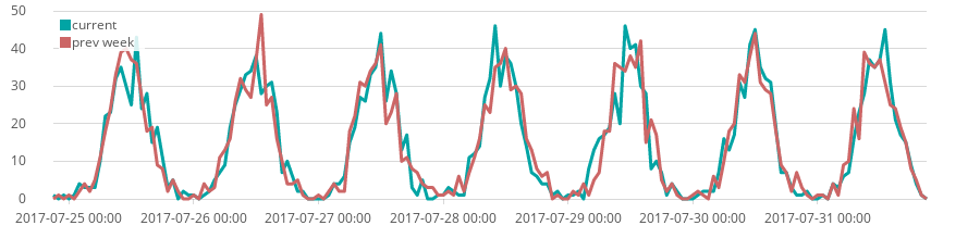
Offsetting data source

Each of the data source functions accept a parameter called offset. It can be used to offset the data by a specific time range. This can be useful to compare data from different time ranges. The offset parameter accepts positive and negative values with a unit. Valid units are s for seconds, m for minutes, h for hours, d for days, w for weeks, M for months and y for years. It will shift the input by the specified offset before drawing it.

To draw our current page visitors (from our sample data) compared to the visits a week before, you can use the following expression:

.es().label(current), .es(offset=-1w).label('prev week')

Styling functions

A few of the functions offered by timelion are used mainly for styling purposes.

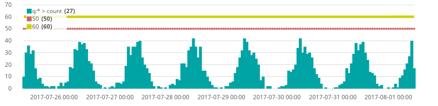
Line style

By default timelion will draw the data with lines. There are three functions to modify the actual graph types: .lines, .bars and .points.

Each of them support a range of parameters to modify e.g. the width of lines, the point sizes, etc. To check all the available parameters have a look at the in-app documentation.

You can see some of the parameters demonstrated in the following expression:

.es().bars(), .static(50).points(symbol=cross, radius=2), .static(60).lines(width=5)

Colors

To manually specify a color for a specific series use the .color function. It expects the color as a HTML color name or a hex value in the #rrggbb format. The following example illustrates the usage:

.es(q=error).color(#FF0000), .es(q=warning).color(yellow)

If you used the split parameter and as such have multiple lines, you can specify multiple colors separated by colon:

.es(split=country:3).color('hotpink:grainsboro:plum')

Math functions

Timelion offers several mathematical calculations on time series.

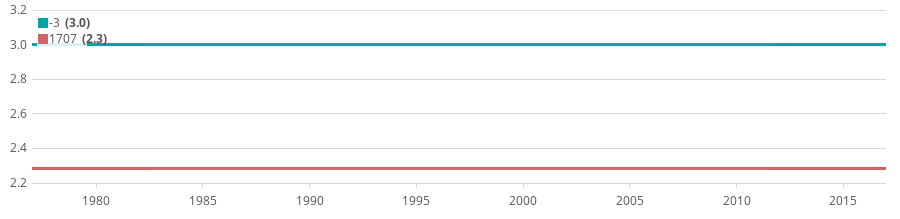
You can chain the .abs function, if you want the y-axis to show the absolute values. You can use the .log function to calculate the logarithm of all values (and optionally specify a logarithmic base).

.static(-5).abs(), .static(1707).log(26)

The .cusum function can be used to calculate the cumulative sum of all values, i.e., the value at a specific point in time is the value of all previous points summed up. Be aware, that the cumulative sum is only calculated from the start time of the graph and not since the dawn of time.

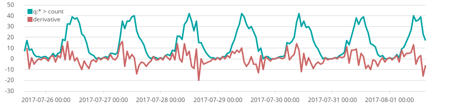
The .derivative function can be used to calculate the derivative of a time series, i.e. the slope of the curve:

.es(), .es().derivative().label(derivative)

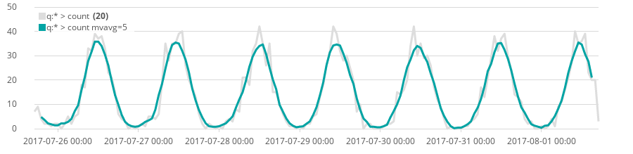
The .mvavg (long .movingaverage) function can be used to smooth series, by applying a moving average to the series. This function requires its first parameter (window), which specifies the size of the window as a value and a time unit (see offsetting above), that is used to calculate the moving average.

The following expression and it result demonstrates the smoothing effect of the moving average:

.es().color(#DDD), .es().mvavg(5h)

Trend

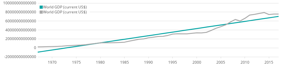
Another useful feature of timelion is the possibility to draw trend lines into a graph. You can use the .trend chaining function on any series, to draw the trend line of that series instead.

To draw a trend line of the world GDP (and the actual world GDP) you can use the following expression:

.wbi(indicator=NY.GDP.MKTP.CD).trend(), .wbi(indicator=NY.GDP.MKTP.CD).color(#AAA)

Different scales

Adding multiple series into one chart will sometimes create the issue, that the values of both series are on completely different scales.

Let's look at the following expression, which draws the GDP of germany (in US$) and the CO2 emission (in metric tons per capita) in one graph:

.wbi(country=de, indicator=NY.GDP.MKTP.CD), .wbi(country=de, indicator=EN.ATM.CO2E.PC)

Luckily these two series are an order of magnitude apart, which would lead in the GDP being clearly visible in the graph and the CO2 emission just being shown as a flatline at the bottom of the graph.

If we are not interested in the actual values, but only in the way the curve changes over time, we can use the .range function to limit a series to a new range of values, i.e. rewriting the minimum and maximum value of the series, but leave the shape intact.

.wbi(country=de, indicator=NY.GDP.MKTP.CD).range(0, 10), .wbi(country=de, indicator=EN.ATM.CO2E.PC).range(0, 10)

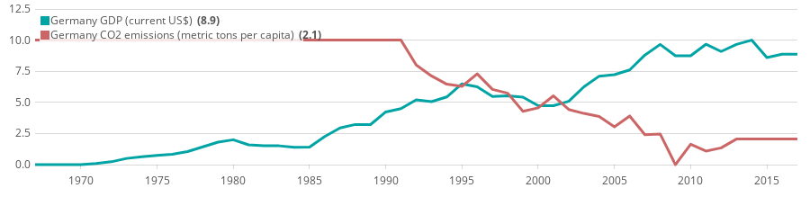
That way we can now see how these two series may or may not correlate. Of course you should never forget, that correlation does not imply causation.

We can simplify the above query, by using timelions grouping functionality, in which we can group multiple series with parentheses and chain a function to the whole group:

(.wbi(country=de, indicator=NY.GDP.MKTP.CD), .wbi(country=de, indicator=EN.ATM.CO2E.PC)).range(0,10)

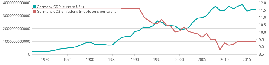
Since we lose the actual values with the range query, in our use case the .yaxis function might be a bit more handy. It will assign a series, to a different y-axis. You have to specify the number of the axis it should be using (with 1 being the default y-axis). It optionally can make use of the min, max, label, color and position parameters, to modify that y-axis.

To achieve now the similar effect as with the .range query, but without losing the actual values, you can use the following expression, to move the two series to different y-axes.

.wbi(country=de, indicator=NY.GDP.MKTP.CD), .wbi(country=de, indicator=EN.ATM.CO2E.PC).yaxis(2)

There is one other scaling issue, that you can hardly solve with classical Kibana virtualizations. Imagine you are drawing the sum of bytes of you server log data. If you watch data from a whole week, each data point on the x-axis will now represent one hour of data, hence have the sum of all bytes transfered within an hour as a value. When selecting a different time range, e.g. four hours, each data point will now only represent a minute, thus having a way lower y-axis value. The following graphs show this situation, with the graph on the left being a time range of a week and the one on the right a time range of four hours. As you can see the y-axis values in the left graph are way higher.

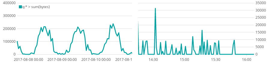
Sometimes that behavior is not what you want, because you might want to compare absolute values with each other no matter what time range you are viewing, or you want these values to be meaningful to you, e.g. because you want to see all values in bytes per second, because you might be used to calculate bandwidth in that unit.

The scaled_interval function does exactly solve that issue. It takes one parameter (named interval), which accepts a time unit (as seen above). Timelion will calculate all values, to be per this interval no matter what time range you are looking. To see the bytes per second, specify a value of 1s, to see the bytes per minute a value of 1m:

.es(metric=sum:bytes).scaled_interval(1s)

This won't change the shape of the graph at all, it will just scale the actual values printed on the y-axis and shown to you when hovering the graph.

Calculate with series

Another of the great advantages in timelion is the ability to calculate with series. You can sum, subtract, multiply or devide series by numbers or even by other series.

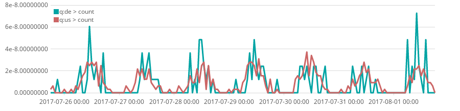
A use case of this is setting information into relation to other informations. If we use our sample webserver data to analyze the visitors from Germany in contrast to the United States, we can use the following expression with the shown result:

.es(de), .es(us)

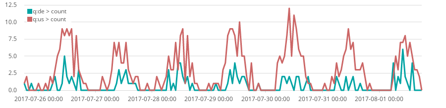
As we can see we have quite some more visitors from the US than from Germany, but of course the US has a significantly higher population than Germany. We can use timelion to divide each series by the actual population of that country, that we pull from World Bank as follows:

.es(de).divide(.wbi(country=de)), .es(us).divide(.wbi(country=us))

We can now see, that we reach in Germany a higher percentage of the population than in the US.

You can use all basic operations via the .add (or .plus), .subtract, .multiply and .divide function. Each accepts either a static value or another series (as in the example above).

Conditional selection

Timelion offers a .min and .max function. These will take a list of multiple series or numeric values, and will always return the minimum of all series/numeric values or maximum (depending on which function you used).

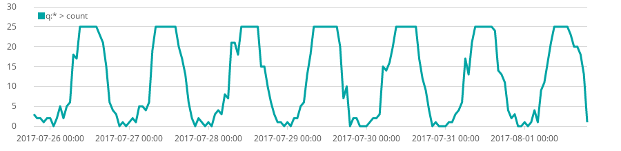
You could that way for example cap a graph at a specific value:

.min(.es(), 25)

Another use case of using .min and .max is coloring graphs conditionally. You could e.g. highlight a series, if it crosses a specific threshold (in this case 25) as follows:

.es().bars(stack=false).color(#F44336), .min(.es(), 25).bars(stack=false).color(#8BC34A)

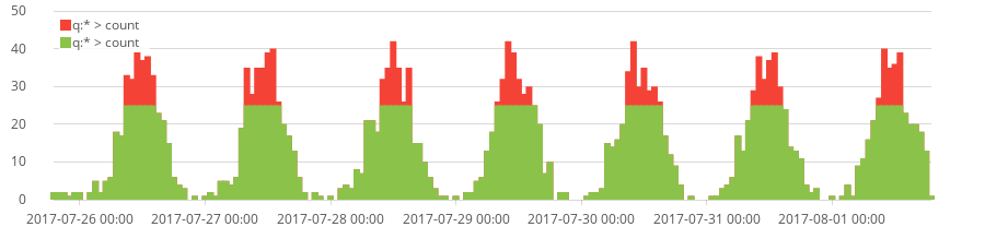
This will first draw the regular .es() data as bars in a red color, and then draw the same data, but capped at 25 in green color. That way the green bars will overdraw the red color and the red bars will only show above a threshold of 25.

If you want a more complex solution for conditional selection, you can use the .if (or long .condition) function to provide a condition and values for the case the condition is true or false.

Rashid Khan posted a great blog post called I have but one .condition(), which explains these functions in detail and show beautiful use cases of their usage.

What's next?

As we've seen in this tutorial timelion offers a wide range of features and possibilities. Some of them cannot be done with classical visualizations, though the feature set of classical visualizations is growing fast - combo charts, pipeline aggregations, and more are just some of the nice new features. It also takes a different approach by using an expression language instead of a classical UI editor.

If you want to continue learning about timelion, I would recommend the Getting Started Guide in the documentation.

If you are trying to do more complex math, Mathlion a free plugin for advanced math calculations in timelion, is worth a look. Davide Bortolami wrote a great blog post about Computation near the visualization layer explaining the background and use cases of Mathlion.

Since Kibana 5.4 an experimental new Time Series Visual Builder has been introduced. It offers a lot of the functionality timelion does (and even some more), but using a graphical editor instead of an expression language. As of Kibana 5.5 timelion and the graphical time series builder are not equivalent feature wise. So you might want to give both a try and see which fit your needs better.