Using deep learning to detect DGAs

The presence of domain names created by a Domain Generation Algorithm (DGA) is a telling indicator of compromise. For example, the domain xeogrhxquuubt.com is a DGA generated domain created by the Cryptolocker ransomware. If a process attempts to connect to this domain, then your network is probably infected with ransomware. Domain blacklists are commonly used in security to prevent connections to such domains, but this blacklisting approach doesn’t generalize to new strains of malware or modified DGA algorithms. We have been researching DGAs extensively at Endgame, and recently posted a paper on arxiv that describes our ability to predict domain generation algorithms using deep learning.

In this blogpost, we’ll briefly summarize our paper, presenting a basic yet powerful technique to detect DGA generated domains that performs far better than “state-of-the-art” techniques presented in academic conferences and journals. “How?” you may ask. Our approach is to use neural networks (more popularly called deep learning) and more specifically, Long Short-Term Memory networks (LSTMs). We’ll briefly discuss the benefits of this specific form of deep learning and then cover our simple yet powerful approach for detecting DGA algorithms.

If you are unfamiliar with machine learning, you may want to jump over to our three part intro series on machine learning before continuing on.

The Benefits of Long Short-Term Memory Networks

Deep learning is a recent buzzword in the machine learning community. Deep learning refers to deeply-layered neural networks (one type of machine learning model), in which feature representations are learned by the model rather than hand-crafted by a user. With roots that go back decades, deep learning has become wildly popular in the last four-five years in large part due to improvements in hardware (such as improved parallel processing with GPUs) and optimization tricks that make training complex networks feasible. LSTMs are one such trick for implementing recurrent neural networks, meaning a neural network that contains cycles. LSTMs are extremely good at learning patterns in long sequences, such as text and speech. In our case, we use them to learn patterns in sequences of characters (domain names) so that we can classify them as DGA-generated or not DGA generated.

The benefit of using deep learning over more conventional machine learning algorithms is that we do not require any feature engineering. Conventional approaches generate a long list of features (such as length, vowel to consonant ratio, and n-gram counts) and use these features to distinguish between DGA-generated and not DGA-generated domains (our colleague wrote about this in a previous post). If an adversary knows your features, they can easily update their DGA to avoid detection. This requires us, as security professionals, to go through a long and arduous process of creating new features to stay ahead. In deep learning, on the other hand, the model learns the feature representations automatically allowing our models to adapt more quickly to an ever-changing adversary.

Another advantage to our technique is that we classify solely on the domain name without the use of any contextual features such as NXDomains and domain reputation. Contextual features can be expensive to generate and often require additional infrastructure (such as network sensors and third party reputations systems). Surprisingly, LSTMs without contextual information perform significantly better than current state of the art techniques that do use contextual information! For those who want to know more about LSTMs, tutorials are plentiful. Two that we recommend: colah’s blog and deeplearning.net, and of course our paper on arxiv.

What is a DGA?

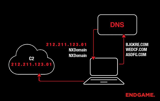
First, a quick note on what a DGA is and why detecting DGAs is important. Adversaries often use domain names to connect malware to command and control servers. These domain names are coded into malware and give the adversary some flexibility in where the C2 is actually hosted in that it’s easy for them to update the domain name to point to a new IP. However, hardcoded domain names are easy to blacklist or sinkhole.

Adversaries use DGAs to evade blacklisting and sinkholing by creating an algorithm (DGA) that creates pseudorandom strings that can be used as domain names. Pseudorandom means that the sequences of strings appear to be random but are actually repeatable given some initial state (or seed). This algorithm is used by both malware that runs on a victim’s machine as well as on some remote software used by the adversary.

On the adversary side, the attacker runs the algorithm and randomly selects a small number of domains (sometimes just one) which he knows will be predicted by the DGA, registers them, and points them at C2 servers. On the victim side, malware runs the DGA and checks an outputted domain to see if it’s live. If a domain is registered, the malware uses this domain as its Command and Control (C2) server. If not, it checks another. This can happen hundreds or thousands of times.

If security researchers gather samples and can reverse engineer the DGA, they can generate lists of all possible domains or pre-register domains which will be predicted in the future and use them for blacklisting or sinkholing, but this doesn’t scale particularly well since thousands or more domains can be generated by a DGA for a given day, with an entirely new list each following day. As you can see, a more generalized approach for predicting whether a given domain name is likely generated by a DGA would be ideal. That generalized approach is what we’re describing here.

Building the LSTM

Training Data

Any machine learning model requires training data. Luckily, training data for this task is easy to find. We used the Alexa top 1 million sites for benign data. We also put together a few DGA algorithms in Python that you can grab on our github site. We use these to generate malicious data. These will generate all the data needed to reproduce the results in this blog.

Tools and Frameworks

We used the Keras toolbox, which is a Python library that makes coding neural networks easy. There are other tools that we like, but Keras is the easiest to demo and understand. Keras is stable and production ready as it uses either Theano or TensorFlow under the hood.

Model Code

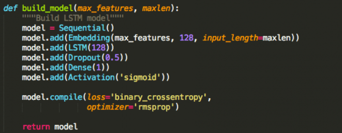
The following is our Python code for building our model:

Yup, that’s it! Here is a very simple breakdown of what we’re doing (with links to additional information):

• We create a basic neural network model on the first line. The next line adds an embedding layer. This layer converts each character into a vector of 128 floats (128 is not a magical number. We chose it as it gave us the best numbers consistently). Each character essentially goes through a lookup once this layer is trained (input character and output 128 floats). max_features defines the number of valid characters. input_length is the maximum length string that we will ever pass to our neural network.
• The next line adds an LSTM layer. This is the main workhorse of our technique. 128 represents the number of dimensions in our internal state (this happens to be the same size as our previous embedding layer by coincidence). More dimensions mean a larger more descriptive model, and we found 128 to work quite well for our task at hand.
• The Dropout layer is a trick used in deep learning to prevent overtraining. You can probably remove this, but we found it useful.
• This Dropout layer precedes a Dense layer (fully connected layer) of size 1.
• We added a sigmoid activation function to squash the output of this layer between 0 and 1, which represent, respectively, benign and malicious.
• We optimize using the cross entropy loss function with the RMSProp optimizer. RMSProp is a variant of stochastic gradient descent and tends to work very well for recurrent neural networks.

Preprocessing Code

Before we start training, we must do some basic data preprocessing. Each string should be converted into an array of ints that represents each possible character. This encoding is arbitrary, but should start at 1 (we reserve 0 for the end-of-sequence token) and be contiguous. An example of how this can be done is given below.

Next, we pad each array of ints to the same length. Padding is a requirement of our toolboxes to better optimize calculations (theoretically, no padding is needed for LSTMs). Fortunately, Keras has a nice function for this:

maxlen represents the length that each array should be. This function pads with 0’s and crops when an array is too long. It’s important that your integer encoding from earlier starts at 1 as the LSTM should learn the difference between padding and characters.

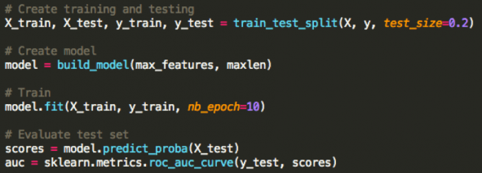
From here, we can divide out our testing and training set, train, and evaluate our performance using a ROC curve.

Comparisons

We compared our simple LSTM technique to three other techniques in our arxiv paper. To keep things simple for this blog, we only compare the results with a single method that uses bigram distributions with logistic regression. This technique also works better than the current state of the art (but not as good as an LSTM) and is surprisingly fast and simple. It is a more conventional feature-based approach where features are the histogram (or raw count) of all bigrams contained within a domain name. The code for this technique is also on our github site.

Results

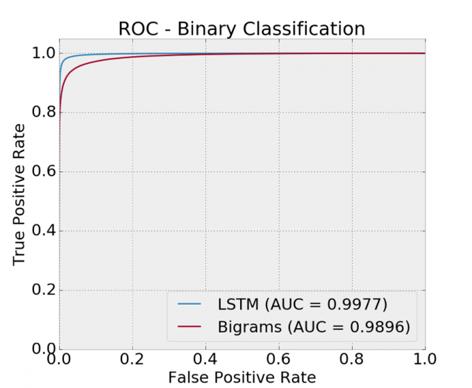
We are finally ready to see some results! And here they are:

Nice! An AUC of 0.9977 with just a few lines of code! All of this is featureless with a simple and straightforward implementation. We actually did a much deeper analysis on a larger and more diverse dataset and observed 90% detection with a 1/10,000 false positive rate, and this can be combined with other approaches outside the scope of this post to improve detection even further. With our LSTM, we even did quite well on multiclass classification, meaning we could classify a piece of malware just by the domains it generated.

Conclusion

We presented a simple technique using neural networks to detect DGAs. The technique uses no contextual information (such as NXDomains or domain reputation) and performs far better than state of the art. While this was a brief summary of our DGA research, feel free to read our complete paper on arxiv and explore our code on github. As always, comments and suggestions are welcome on our github site!