From vector search to powerful REST APIs, Elasticsearch offers developers the most extensive search toolkit. Dive into our sample notebooks in the Elasticsearch Labs repo to try something new. You can also start your free trial or run Elasticsearch locally today.
We have supported float values from the beginning of vector search in Elasticsearch. In version 8.6, we added support for byte encoded vectors. In 8.14, we added automatic quantization down to half-byte values. In 8.15, we are adding support for bit encoded vectors.
But what are bit vectors and their practical implications? As stated on the tin, bit vectors are where each dimension of the vector is a single bit. When comparing data sizes for vectors with the typical float values, bit vectors provide a whopping 32x reduction in size.
Every bit counts
Some semantic embedding models natively output bit vectors such as Cohere. Additionally, some other kinds of data such as image hashing utilize bit vectors directly.
However, most semantic embedding models output float vectors and do not support bit encoding directly.
You can naively binarize vectors yourself since the math is simple. For each vector dimension, check if the value is > median. If it is, that is a 1 bit, and otherwise it is a 0 bit.
Figure 0: Transforming 8 float values into individual bit values and then collapse to single byte, assuming the median value is 0.
Here is some simple Python code to binarize a vector:
Obviously, this can lose a fair bit of information (pun intended). But for larger vectors or vectors specifically optimized to work well with bit encoding, the space savings can be worth it.
Consider 1 million 1024 dimension floating point vectors. Each vector is 4KB in size and all vectors will require approximately 4GB. With binary quantization, each vector is now only 128 bytes and all vectors in total are only around 128MB. When you consider the cost of storage & memory, this is exceptionally attractive.
Now, since we are no longer in float land, we cannot use typical distance functions like cosineSimilarity or dotProduct. Instead, we take advantage of each dimension being a single bit by using Hamming distance.
hamming distance is fairly straight forward, for every individual bit, we calculate the xor with the corresponding bit in the other vector. Then we sum up the resulting bits.
Figure 1: Hamming distance calculation between two bit elements.
Let's think back to our 1 million 1024 dimension vectors. In addition to the space savings, using hamming distance over 128 bytes vs. dotProduct over 1024 floats is a significant reduction in computation time.
For some simple benchmarking (this is not exhaustive), we indexed 1 million 1024 dimension vectors in Elasticsearch with a flat index.
With only 2GB of off-heap, bit vectors take approximately 40ms to return, but float takes over 3000ms. If we increase the off-heap to 4GB, bit vectors continue to take the same amount of time (they fit into memory even before) and float vectors improve to 200ms.
So hamming is still significantly faster than the floating point dot-product and requires significantly less memory.
A bit of error
bit vectors aren't perfect, it is obvious that it is a lossy encoding. The concern isn't that vectors will not be unique. Even when using a bit encoding, 386 dimensioned vectors still have possible unique vectors. The main concerns are distance collisions and the size of the error the encoding introduces.
Even if we assume a well distributed bit encoding, it's likely to have many distance collisions when gathering a large number of vectors. Intuitively, this makes sense as our distance measurement is summing the bits. For example, 00000001 and 10000000 are the same distance apart as 00000001 and 00000010. Once you need to gather more than dimension documents, you will have collisions. In reality, it will occur much sooner than that.
To illustrate, here is a small study. The focus here is finding out how many bit vectors would need gathering to get the true nearest top vectors.
For the first experiment, we used 1 million CohereV3 vectors from their Wikipedia dataset. We randomly sampled (without replacement) 50 query vectors and used those to determine true dotProduct and hamming distances.
Here are the "best" and "worst" performing query vectors. With quality being the number of documents required to retrieve the correct nearest neighbors (e.g. more being worse).

Figure 2: The best performing CohereV3 query vector & its distances, you can see how the distances are actually aligning well.

Figure 3: The worst performing CohereV3 query vector & its distances. Here, the nearer distances align well, but that correlation weakens as we start gathering vectors that are further away.

Figure 4: The median number of vectors required to get the true nearest neighbors over all 50 queries. CohereV3 is excellent here, showing that only around 10x oversampling is required, even for the nearest neighbor. Visually, however, we can see that the oversampling required increases exponentially.
From this small study, CohereV3 does exceptionally well. The median case showing you can oversample by approximately 10x to achieve similar recall. However, in the worst case when gathering more than 50 nearest documents, it starts being problematic, requiring much more than 10x oversampling. Depending on the query and the dataset you can run into problems.
So, how well does binarization do when a model and dataset combination are not optimized for bit vectors? We used e5-small-v2 and embedded the quora datset to test this. Randomly taking 500k vectors and then randomly sampled 50 query vectors from those vectors.

Figure 5: The best performing e5-small query vector & its distances. The extremely near distances align fairly well, but still not exceptionally so.

Figure 6: The worst performing e5-small query vector & its distances. The hamming and dotProduct distances are effectively uncorrelated.

Figure 7: The median number of vectors required to get the true nearest neighbors.
The best e5-small vector does moderately well and its hamming distances are semi-correlated with the dotProduct. The worst case is a drastically different story. The distances are effectively uncorrelated. The median values show that you would need to oversample by approximately 800x to achieve the nearest 10 vectors and it only gets worse from there.
In short, for models that do well with binary quantization and when the model is well adapted to the dataset, bit quantization is a great option. That said, keep in mind that the oversampling required can increase exponentially as you gather more vectors.
For out-of-domain data sets where nearest vectors are not well distinguished for the model, or for models that are not optimized for binary quantization at all, bit vectors can be problematic, even with a small number of nearest vectors.
Ok, but how do I use
When using bit vectors in Elasticsearch, you can specify the bit encoding in the mapping. For example:
Figure 8: Mapping a bit vector in Elasticsearch, allowing for bit encoding. The first document will statically set the bit dimensions
Or if you do not want to index in the HNSW index, you can use the flat index type.
Figure 9: Mapping a bit vector in Elasticsearch in a flat index type.
Then, to index a document with a bit vector, you can use the following:
Figure 10: A 1024 dimensioned bit vector in hexidecimal format.
Now you can utilize a knn query
Figure 11: Querying bit vectors with a 1024 dimensioned hexidecimal vector.
Just a bit more
Thank you for making it through all the 2-bit jokes. We are very excited about the possibilities that bit vectors bring to Elasticsearch in 8.15. Please try it out in Elastic Cloud once 8.15 is released or in Elasticsearch Serverless right now!
Frequently Asked Questions
What are bit vectors in Elasticsearch?
`Bit vectors are where each dimension of the vector is a single bit. When comparing data sizes for vectors with the typical `float` values, bit vectors provide a whopping 32x reduction in size.
Related Content
March 2, 2026
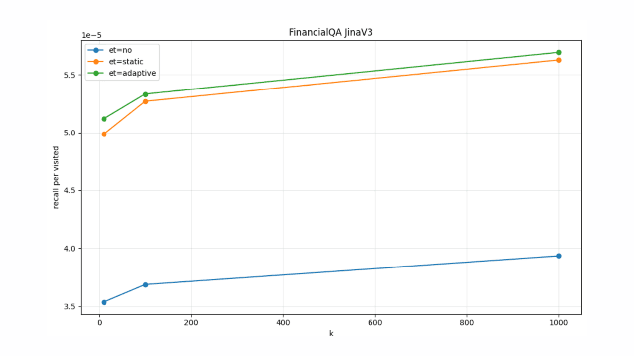
Adaptive early termination for HNSW in Elasticsearch
Introducing a new adaptive early termination strategy for HNSW in Elasticsearch.
February 25, 2026
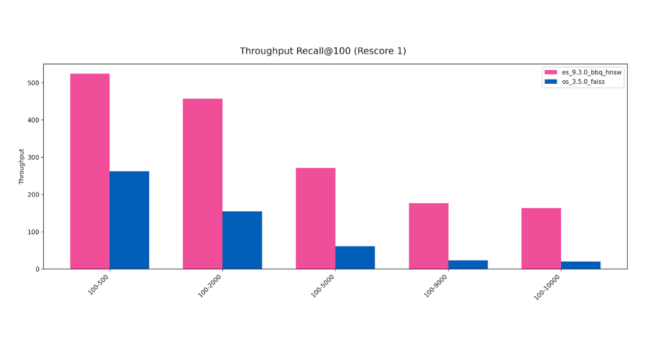
Elasticsearch vector search is up to 8x faster than OpenSearch
Exploring filtered vector search benchmarks of OpenSearch vs. Elasticsearch and why vector search performance is critical for context-engineered systems.
February 16, 2026
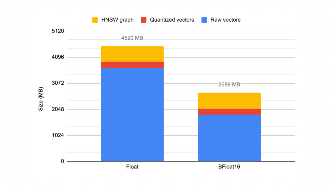
Elasticsearch 9.3 adds bfloat16 vector support
Exploring the new Elasticsearch element_type: bfloat16, which can halve your vector data storage.
February 10, 2026
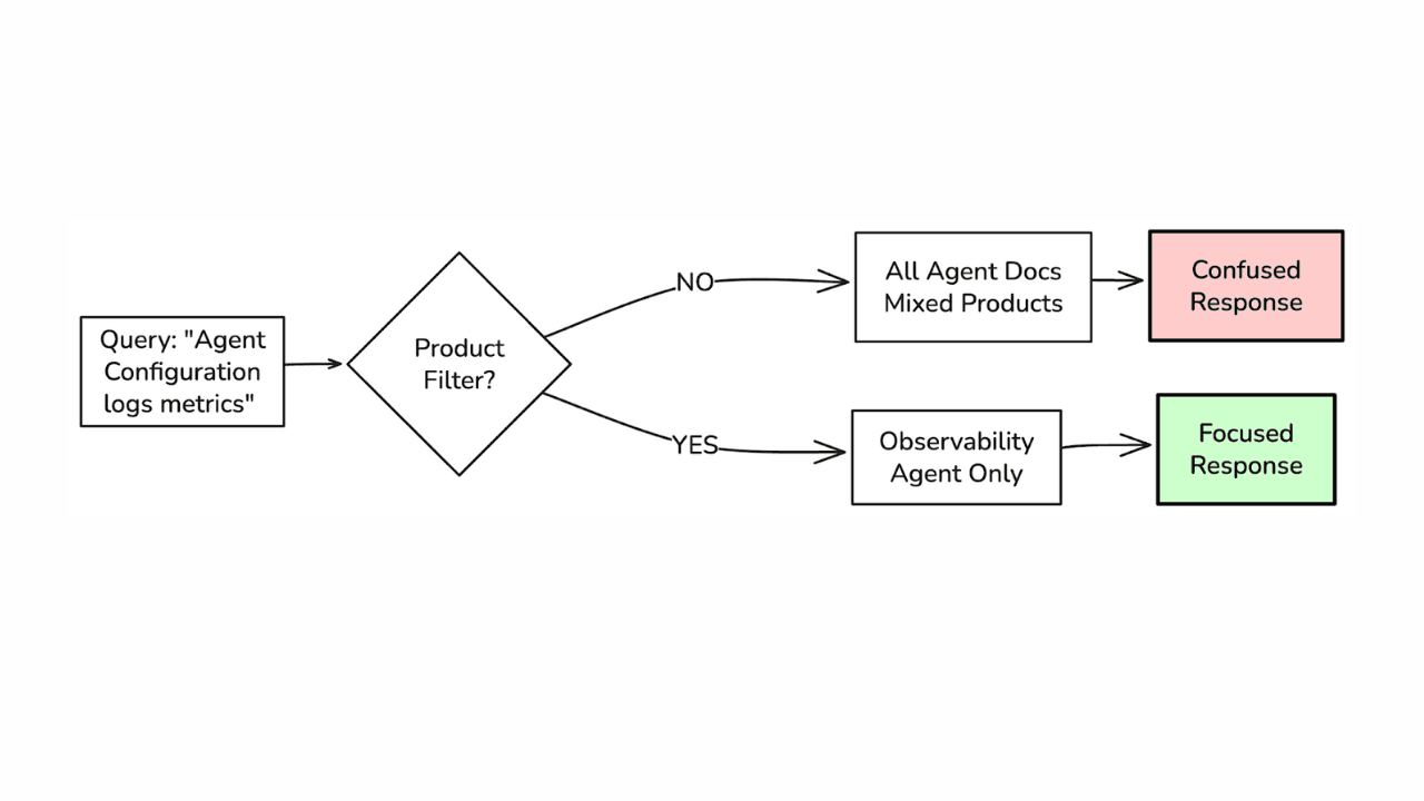
How to defend your RAG system from context poisoning
How context engineering techniques prevent context poisoning in LLM responses.
February 4, 2026
Speed up vector ingestion using Base64-encoded strings
Introducing Base64-encoded strings to speed up vector ingestion in Elasticsearch.