From vector search to powerful REST APIs, Elasticsearch offers developers the most extensive search toolkit. Dive into our sample notebooks in the Elasticsearch Labs repo to try something new. You can also start your free trial or run Elasticsearch locally today.
Part 1: High-fidelity dense vector search
Introduction
When designing for a vector search experience, the sheer number of available options can feel overwhelming. Initially, managing a small number of vectors is straightforward, but as applications scale, this can quickly become a bottleneck.
In this blog post series, we’ll explore the cost and performance of running large-scale vector search with Elasticsearch across various datasets and use cases.
We begin the series with one of the largest publicly available vector datasets: the Cohere/msmarco-v2-embed-english-v3. This dataset includes 138 million passages extracted from web pages in the MSMARCO-passage-v2 collection, embedded into 1024 dimensions using Cohere's latest embed-english-v3 model.
For this experiment, we defined a reproducible track that you can run on your own Elastic deployment to help you benchmark your own high fidelity dense vector search experience.
It is tailored for real-time search use cases where the latency of a single search request must be low (<100ms). It uses Rally, our open source tool, to benchmark across Elasticsearch versions.
In this post, we use our default automatic quantization for floating point vectors. This reduces the RAM cost of running vector searches by 75% without compromising retrieval quality. We also provide insights into the impact of merging and quantization when indexing billions of dimensions.
We hope this track serves as a useful baseline, especially if you don’t have vectors specific to your use case at hand.
Notes on embeddings
Picking the right model for your needs is outside the scope of this blog post but in the next sections we discuss different techniques to compress the original size of your vectors.
Matryoshka Representation Learning (MRL)
By storing the most important information in earlier dimensions, new methods like Matryoshka embeddings can shrink dimensions while keeping good search accuracy. With this technique, certain models can be halved in size and still maintain 90% of their NDCG@10 on MTEB retrieval benchmarks. However, not all models are compatible. If your chosen model isn't trained for Matryoshka reduction or if its dimensionality is already at its minimum, you'll have to manage dimensionality directly in the vector database.
Fortunately, the latest models from mixedbread or OpenAI come with built-in support for MRL.
For this experiment we choose to focus on a use case where the dimensionality is fixed (1024 dimensions), playing with the dimensionality of other models will be the topic for another time.
Embedding quantization learning
Model developers are now commonly offering models with various trade-offs to address the expense of high-dimensional vectors. Rather than solely focusing on dimensionality reduction, these models achieve compression by adjusting the precision of each dimension.
Typically, embedding models are trained to generate dimensions using 32-bit floating points. However, training them to produce dimensions with reduced precision helps minimize errors. Developers usually release models optimized for well-known precisions that directly align with native types in programming languages.
For example, int8 represents a signed integer ranging from -127 to 127, while uint8 denotes an unsigned integer ranging from 0 to 255. Binary, the simplest form, represents a bit (0 or 1) and corresponds to the smallest possible unit per dimension.
Implementing quantization during training allows for fine-tuning the model weights to minimize the impact of compression on retrieval performance. However, delving into the specifics of training such models is beyond the scope of this blog.
In the following section, we will introduce a method for applying automatic quantization if the chosen model lacks this feature.
Adaptive embedding quantization
In cases where models lack quantization-aware embeddings, Elasticsearch employs an adaptive quantization scheme that defaults to quantizing floating points to int8.
This generic int8 quantization typically results in negligible performance loss. The benefit of this quantization lies in its adaptability to data drift.
It utilizes a dynamic scheme where quantization boundaries can be recalculated from time to time to accommodate any shifts in the data.
Large scale benchmark
Back-of-the-envelope estimation
With 138.3 million documents and 1024-dimensional vectors, the raw size of the MSMARCO-v2 dataset to store the original float vectors exceeds 520GB. Using brute force to search the entire dataset would take hours on a single node.
Fortunately, Elasticsearch offers a data structure called HNSW (Hierarchical Navigable Small World Graph), designed to accelerate nearest neighbor search. This structure allows for fast approximate nearest neighbor searches but requires every vector to be in memory.
Loading these vectors from disk is prohibitively expensive, so we must ensure the system has enough memory to keep them all in memory.
With 1024 dimensions at 4 bytes each, each vector requires 4 kilobytes of memory.
Additionally, we need to account for the memory required to load the Hierarchical Navigable Small World (HNSW) graph into memory. With the default setting of 32 neighbors per node in the graph, an extra 128 bytes (4 bytes per neighbor) of memory per vector is necessary to store the graph, which is equivalent to approximately 3% of the memory cost of storing the vector dimensions.
Ensuring sufficient memory to accommodate these requirements is crucial for optimal performance.
On Elastic Cloud, our vector search-optimized profile reserves 25% of the total node memory for the JVM (Java Virtual Machine), leaving 75% of the memory on each data node available for the system page cache where vectors are loaded. For a node with 60GB of RAM, this equates to 45GB of page cache available for vectors. The vector search optimized profile is available on all Cloud Solution Providers (CSP) AWS, Azure and GCP.
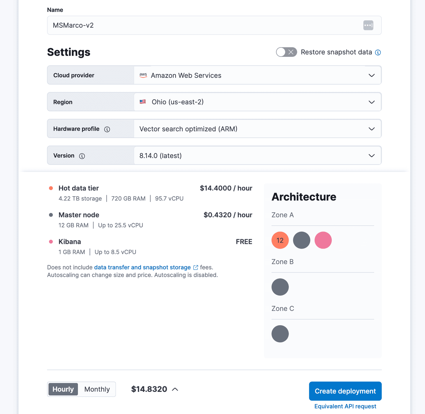
To accommodate the 520GB of memory required, we would need 12 nodes, each with 60GB of RAM, totaling 720GB.
At the time of this blog this setup can be deployed in our Cloud environment for a total cost of $14.44 per hour on AWS: (please note that the price will vary for Azure and GCP environments):
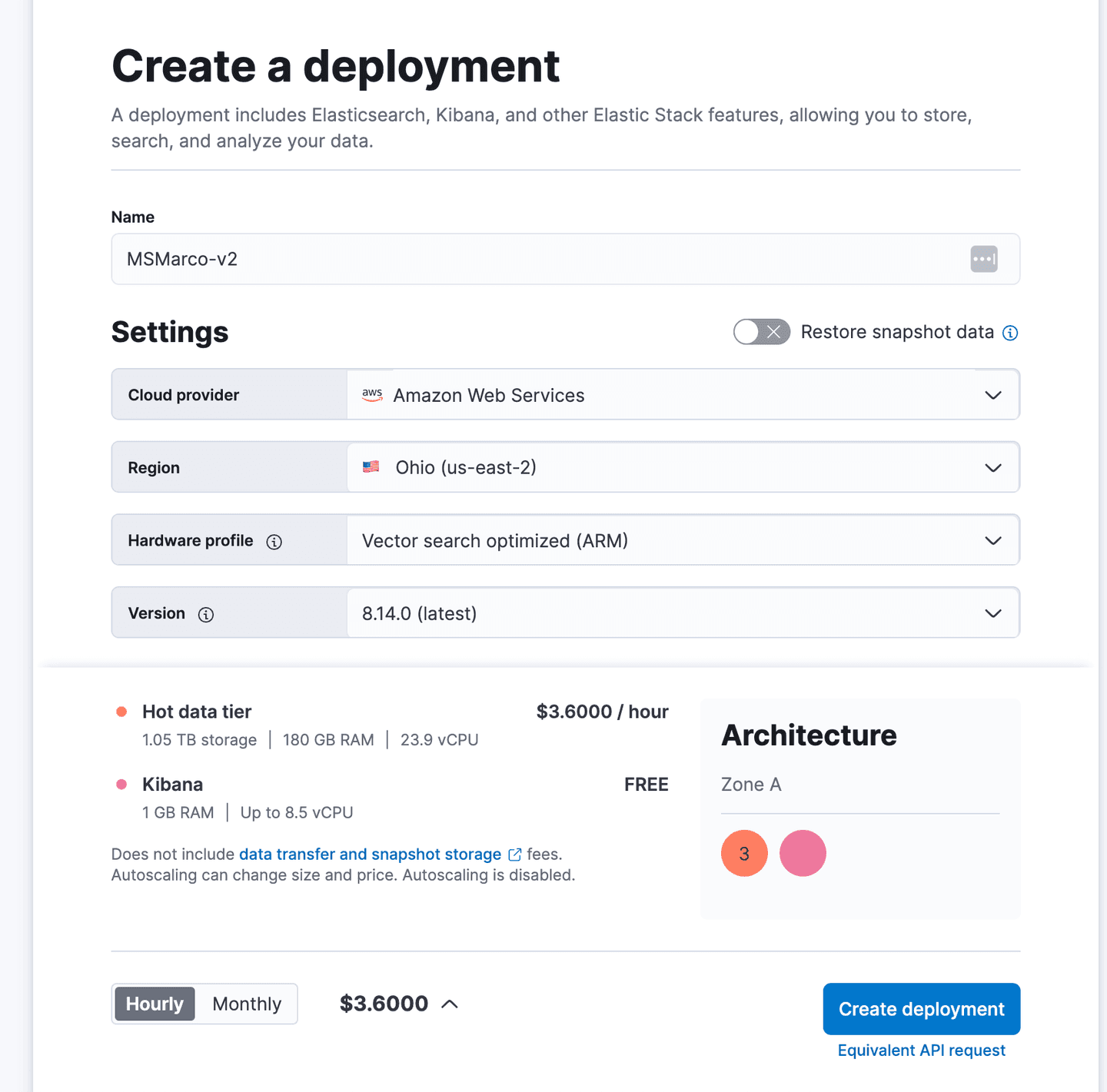
By leveraging auto-quantization to bytes, we can reduce the memory requirement to 130gb, which is just a quarter of the original size.
Applying the same 25/75 memory allocation rule, we can allocate a total of 180 gb of memory on Elastic Cloud.
At the time of this blog this optimized setup results in a total cost of $3.60 per hour on Elastic Cloud (please note that the price will vary for Azure and GCP environments):
Start a free trial on Elastic Cloud and simply select the new Vector Search optimized profile to get started.
In this post, we'll explore this cost-effective quantization using the benchmark we created to experiment with large-scale vector search performance. By doing so, we aim to demonstrate how you can achieve significant cost savings while maintaining high search accuracy and efficiency.
Benchmark configuration
The msmarco-v2-vector rally track defines the default mapping that will be used.
It includes one dense vector field with 1024 dimensions, indexed with auto int8 quantization, and a doc_id field of type keyword to uniquely identify each passage.
For this experiment, we tested with two configurations:
- Default: This serves as the baseline, using the track on Elasticsearch with default options.
- Aggressive Merge: This configuration provides a comparison point with different trade-offs.
As previously explained, each shard in Elasticsearch is composed of segments. A segment is an immutable division of data that contains the necessary structures to directly lookup and search the data.
Document indexing involves creating segments in memory, which are periodically flushed to disk.
To manage the number of segments, a background process merges segments to keep the total number under a certain budget.
This merge strategy is crucial for vector search since HNSW graphs are independent within each segment. Each dense vector field search involves finding the nearest neighbors in every segment, making the total cost dependent on the number of segments.
By default, Elasticsearch merges segments of approximately equal size, adhering to a tiered strategy controlled by the number of segments allowed per tier.
The default value for this setting is 10, meaning each level should have no more than 10 segments of similar size. For example, if the first level contains segments of 50MB, the second level will have segments of 500MB, the third level 5GB, and so on.
The aggressive merge configuration adjusts the default settings to be more assertive:
- It sets the segments per tier to 5, enabling more aggressive merges.
- It increases the maximum merged segment size from 5GB to 25GB to maximize the number of vectors in a single segment.
- It sets the floor segment size to 1GB, artificially starting the first level at 1GB.
With this configuration, we expect faster searches at the expense of slower indexing.
For this experiment, we kept the default settings for m, ef_construction, and confidence_interval options of the HNSW graph in both configurations. Experimenting with these indexing parameters will be the subject of a separate blog. In this first part, we chose to focus on varying the merge and search parameters.
When running benchmarks, it's crucial to separate the load driver, which is responsible for sending documents and queries, from the evaluated system (Elasticsearch deployment). Loading and querying hundreds of millions of dense vectors require additional resources that would interfere with the searching and indexing capabilities of the evaluated system if run together.
To minimize latency between the system and the load driver, it's recommended to run the load driver in the same region of the Cloud provider as the Elastic deployment, ideally in the same availability zone.
For this benchmark, we provisioned an im4gn.4xlarge node on AWS with 16 CPUs, 64GB of memory, and 7.5TB of disk in the same region as the Elastic deployment. This node is responsible for sending queries and documents to Elasticsearch. By isolating the load driver in this manner, we ensure accurate measurement of Elasticsearch's performance without the interference of additional resource demands.
We ran the entire benchmarks with the following configuration:
The initial_indexing_bulk_indexing_clients value of 12 indicates that we will ingest data from the load driver using 12 clients. With a total of 23.9 vCPUs in the Elasticsearch data nodes, using more clients to send data increases parallelism and enables us to fully utilize all available resources in the deployment.
For search operations, the standalone_search_clients and parallel_indexing_search_clients values of 8 mean that we will use 8 clients to query Elasticsearch in parallel from the load driver. The optimal number of clients depends on multiple factors; in this experiment, we selected the number of clients to maximize CPU usage across all Elasticsearch data nodes.
To compare the results, we ran a second benchmark on the same deployment, but this time we set the parameter aggressive_merge to true. This effectively changes the merge strategy to be more aggressive, allowing us to evaluate the impact of this configuration on search performance and indexing speed.
Indexing performance
In Rally, a challenge is configured with a list of scheduled operations to execute and report.
Each operation is responsible for performing an action against the cluster and reporting the results.
For our new track, we defined the first operation as initial-documents-indexing, which involves bulk indexing the entire corpus. This is followed by wait-until-merges-finish-after-index, which waits for background merges to complete at the end of the bulk loading process.
This operation does not use force merge; it simply waits for the natural merge process to finish before starting the search evaluation.
Below, we report the results of these operations of the track, they correspond to the initial loading of the dataset in Elasticsearch. The search operations are reported in the next section.
With Elasticsearch 8.14.0, the initial indexing of the 138M vectors took less than 5 hours, achieving an average rate of 8,000 documents per second.
Please note that the bottleneck is typically the generation of the embeddings, which is not reported here.
Waiting for the merges to finish at the end added only 2 extra minutes:
Total Indexing performance (8.14.0 default int8 HNSW configuration)

For comparison, the same experiment conducted on Elasticsearch 8.13.4 required almost 6 hours for ingestion and an additional 2 hours to wait for merges:
Total Indexing performance (8.13.4 default int8 HNSW configuration)

Elasticsearch 8.14.0 marks the first release to leverage native code for vector search. A native Elasticsearch codec is employed during merges to accelerate similarities between int8 vectors, leading to a significant reduction in overall indexing time. We're currently exploring further optimizations by utilizing this custom codec for searches, so stay tuned for updates!
The aggressive merge run completed in less than 6 hours, averaging 7,000 documents per second. However, it required nearly an hour to wait for merges to finish at the end. This represents a 40% decrease in speed compared to the run with the default merge strategy:
Total Indexing performance (8.14.0 aggressive merge int8 HNSW configuration)

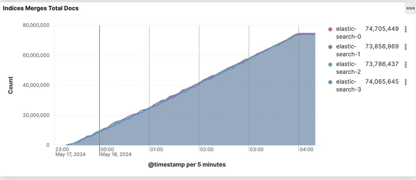
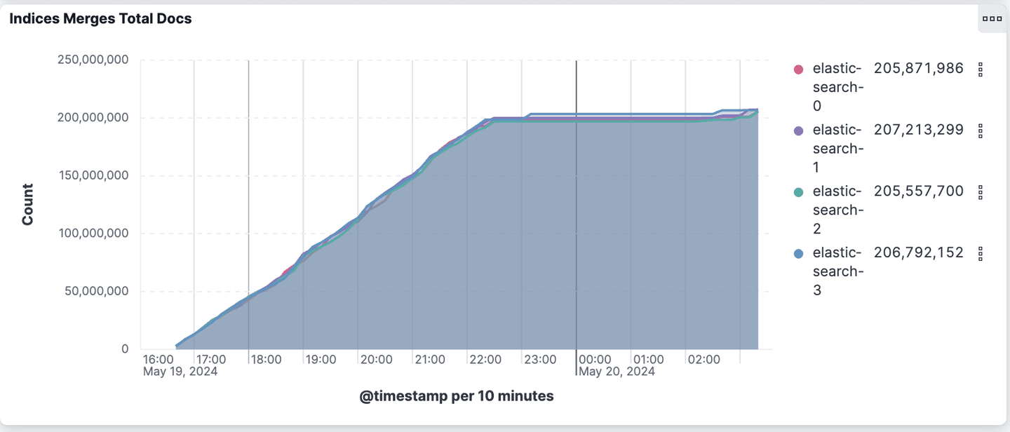
This additional work performed by the aggressive merge configuration can be summarized in the two charts below.
The aggressive merge configuration merges 2.7 times more documents to create larger and fewer segments. The default merge configuration reports nearly 300 million documents merged from the 138 million documents indexed. This means each document is merged an average of 2.2 times.
Total number of merged documents per node (8.14.0 default int8 HNSW configuration)
Total number of merged documents per node (8.14.0 aggressive merge int8 HNSW configuration)
In the next section we’ll analyze the impact of these configurations on the search performance.
Search evaluation
For search operations, we aim to capture two key metrics: the maximum query throughput and the level of accuracy for approximate nearest neighbor searches.
To achieve this, the standalone-search-knn-* operations evaluate the maximum search throughput using various combinations of approximate search parameters. This operation involves executing 10,000 queries from the training set using parallel_indexing_search_clients in parallel as rapidly as possible. These operations are designed to utilize all available CPUs on the node and are performed after all indexing and merging tasks are complete.
To assess the accuracy of each combination, the knn-recall-* operations compute the associated recall and Normalized Discounted Cumulative Gain (nDCG). The nDCG is calculated from the 76 queries published in msmarco-passage-v2/trec-dl-2022/judged, using the 386,000 qrels annotations. All nDCG values range from 0.0 to 1.0, with 1.0 indicating a perfect ranking.
Due to the size of the dataset, generating ground truth results to compute recall is extremely costly. Therefore, we limit the recall report to the 76 queries in the test set, for which we computed the ground truth results offline using brute force methods.
The search configuration consists of three parameters:
- k: The number of passages to return.
- num_candidates: The size of the queue used to limit the search on the nearest neighbor graph.
- num_rescore: The number of passages to rescore using the full fidelity vectors.
Using automatic quantization, rescoring slightly more than k vectors with the original float vectors can significantly boost recall.
The operations are named according to these three parameters. For example, knn-10-100-20 means k=10, num_candidates=100, and num_rescore=20. If the last number is omitted, as in knn-10-100, then num_rescore defaults to 0.
See the track.py file for more information on how we create the search requests.
The chart below illustrates the expected Queries Per Second (QPS) at different recall levels. For instance, the default configuration (the orange series) can achieve 50 QPS with an expected recall of 0.922.
Recall versus Queries Per Second (Elasticsearch 8.14.0)
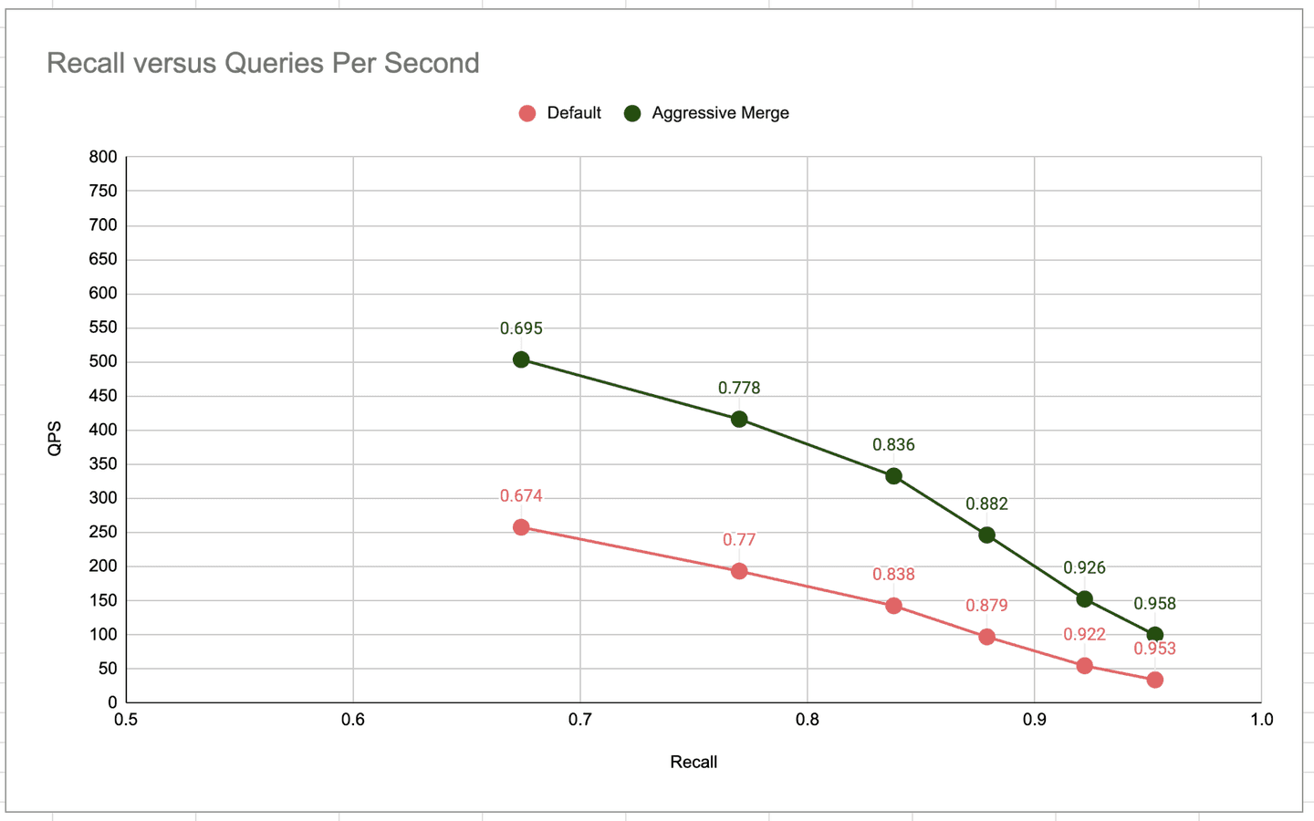
The aggressive merge configuration is 2 to 3 times more efficient for the same level of recall. This efficiency is expected since the search is conducted on larger and fewer segments as demonstrated in the previous section.
The full results for the default configuration are presented in the table below:
Queries per second, latencies (in milliseconds), recall and NDCG@10 with different parameters combination (8.14 default int8 HNSW configuration)
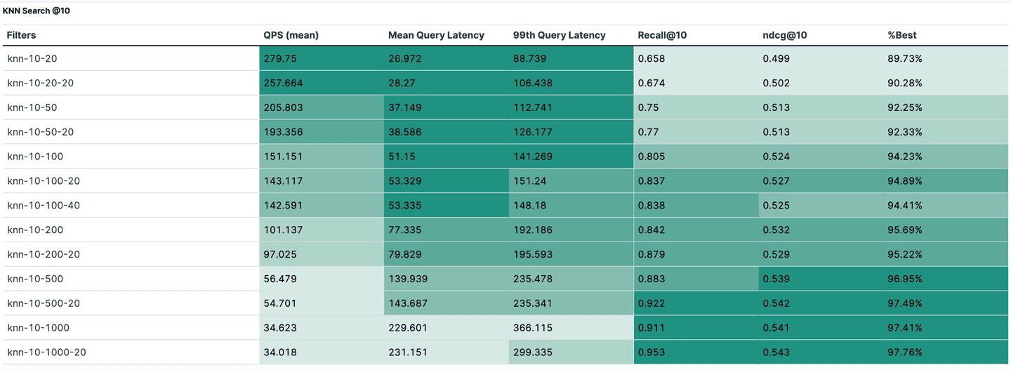
The %best column represents the difference between the actual NDCG@10 for this configuration and the best possible NDCG@10, determined using the ground truth nearest neighbors computed offline with brute force.
For instance, we observe that the knn-10-20-20 configuration, despite having a recall@10 of 67.4%, achieves 90% of the best possible NDCG for this dataset. Note that this is just a point result and results may vary with other models and/or datasets.
The table below shows the full results for the aggressive merge configuration:
Queries per second, latencies (in milliseconds), recall and NDCG@10 with different parameters combination (8.14 aggressive merge int8 HNSW configuration)
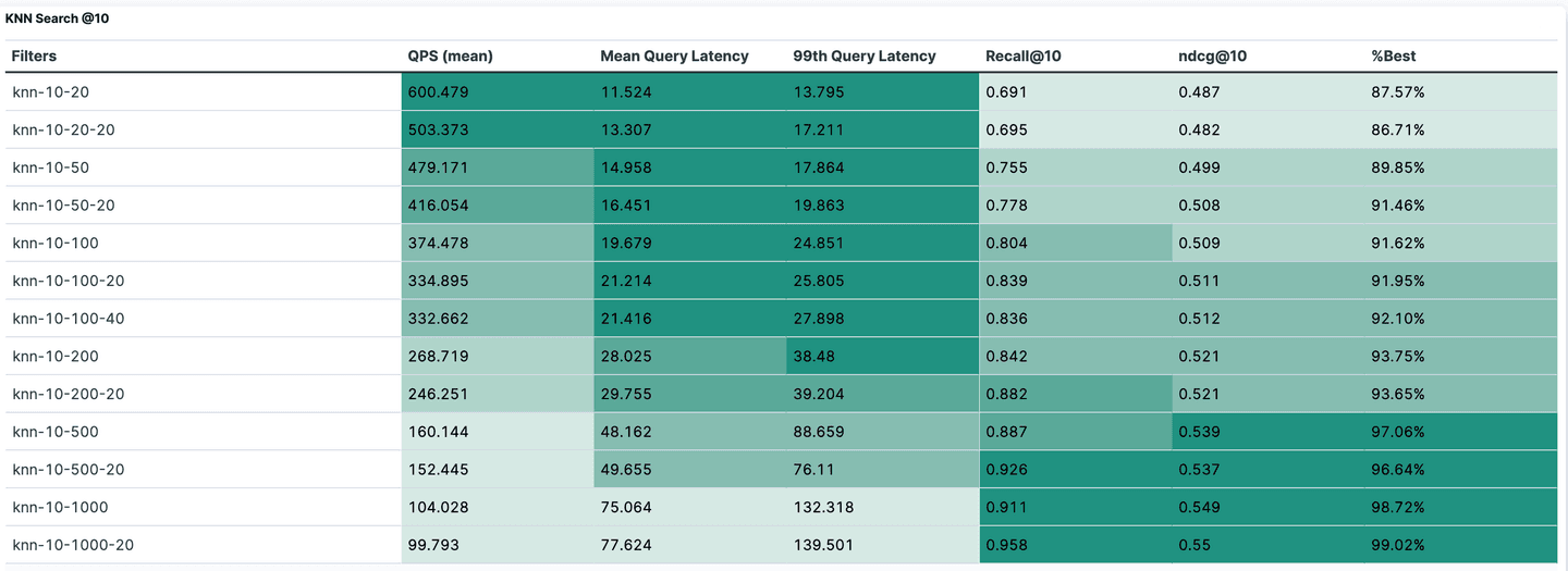
Using the knn-10-500-20 search configuration, the aggressive merge setup can achieve > 90% recall at 150 QPS.
Conclusion
In this post, we described a new rally track designed to benchmark large-scale vector search on Elasticsearch. We explored various trade-offs involved in running an approximate nearest neighbor search and demonstrated how in Elasticsearch 8.14 we've reduced the cost by 75% while increasing index speed by 50% for a realistic large scale vector search workload.
Our ongoing efforts focus on optimization and identifying opportunities to enhance our vector search capabilities. Stay tuned for the next installment of this series, where we will delve deeper into the cost and efficiency of vector search use cases, specifically examining the potential of int4 and binary compression techniques.
By continually refining our approach and releasing tools for testing performance at scale, we aim to push the boundaries of what is possible with Elasticsearch, ensuring it remains a powerful and cost-effective solution for large-scale vector search.
Related Content
February 16, 2026
Elasticsearch 9.3 adds bfloat16 vector support
Exploring the new Elasticsearch element_type: bfloat16, which can halve your vector data storage.
February 10, 2026
How to defend your RAG system from context poisoning
How context engineering techniques prevent context poisoning in LLM responses.
February 4, 2026
Speed up vector ingestion using Base64-encoded strings
Introducing Base64-encoded strings to speed up vector ingestion in Elasticsearch.

February 5, 2026
ES|QL dense vector search support
Using ES|QL for vector search on your dense_vector data.

January 28, 2026
Apache Lucene 2025 wrap-up
2025 was a stellar year for Apache Lucene; here are our highlights.