Get hands-on with Elasticsearch: Dive into our sample notebooks in the Elasticsearch Labs repo, start a free cloud trial, or try Elastic on your local machine now.
Elasticsearch has had powerful geospatial search and analytics capabilities for many years, but the API was quite different from what typical GIS users were used to. In the past year we've added the ES|QL query language, a piped query language as easy, or even easier, than SQL. It's particularly suited to the search, security, and observability use cases Elastic excels at. We're also adding support for geospatial search and analytics within ES|QL, making it far easier to use, especially for users coming from SQL or GIS communities.
Elasticsearch 8.12 and 8.13 brought basic support for geospatial types to ES|QL. This was dramatically enhanced with the addition of geospatial search capabilities in 8.14. More importantly, this support was designed to conform closely to the Simple Feature Access standard from the Open Geospatial Consortium (OGC) used by other spatial databases like PostGIS, making it much easier to use for GIS experts familiar with these standards.
In this blog, we'll show you how to use ES|QL to perform geospatial searches, and how it compares to the SQL and Query DSL equivalents. We'll also show you how to use ES|QL to perform spatial joins, and how to visualize the results in Kibana Maps. Note that all the features described here are in "technical preview", and we'd love to hear your feedback on how we can improve them.
Searching for geospatial data
Let's start with an example query:
This performs a search for any city boundary polygons that intersect with a rectangular search polygon around the Sanya Phoenix International Airport (SYX).
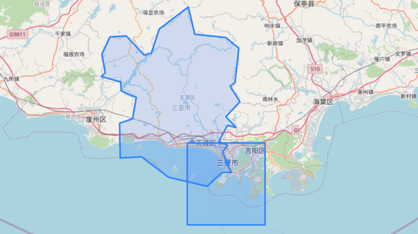
In a sample dataset of airports, cities and city boundaries, this search finds the intersecting polygon and returns the desired fields from the matching document:
| abbrev | airport | region | city | city_location |
|---|---|---|---|---|
| SYX | Sanya Phoenix Int'l | 天涯区 | Sanya | POINT(109.5036 18.2533) |
That was easy! Now compare this to the classic Elasticsearch Query DSL for the same query:
Both queries are reasonably clear in their intent, but the ES|QL query closely resembles SQL. The same query in PostGIS looks like this:
Look back at the ES|QL example. So similar, right?
We've found that existing users of the Elasticsearch API find ES|QL much easier to use. We now expect that existing SQL users, particularly Spatial SQL users, will find that ES|QL feels very familiar to what they are used to seeing.
Why not SQL?
What about Elasticsearch SQL? It has been around for a while and has some geospatial features. However, Elasticsearch SQL was written as a wrapper on top of the original Query API, which meant only queries that could be transpiled down to the original API were supported. ES|QL does not have this limitation. Being a completely new stack allows for many optimizations that were not possible in SQL. Our benchmarks show ES|QL is very often faster than the Query API, particularly with aggregations!
Differences to SQL
Clearly, from the previous example, ES|QL is somewhat similar to SQL, but there are some important differences. For example, ES|QL is a piped query language, starting with a source command like FROM and then chaining all subsequent commands together with the pipe | character. This makes it very easy to understand how each command receives a table of data and performs some action on that table, such as filtering with WHERE, adding columns with EVAL, or performing aggregations with STATS. Rather than starting with SELECT to define the final output columns, there can be one or more KEEP commands, with the last one specifying the final output results. This structure simplifies reasoning about the query.
Focusing in on the WHERE command in the above example, we can see it looks quite similar to the PostGIS example:
ES|QL
PostGIS
Aside from the difference in string quotation characters, the biggest difference is in how we type-cast the string to a spatial type. In PostGIS, we use the ::geometry suffix, while in ES|QL, we use the ::geo_shape suffix. This is because ES|QL runs within Elasticsearch, and the type-casting operator :: can be used to convert a string to any of the supported ES|QL types, in this case, a geo_shape. Additionally, the geo_shape and geo_point types in Elasticsearch imply the spatial coordinate system known as WGS84, more commonly referred to using the SRID number 4326. In PostGIS, this needs to be explicit, hence the use of the SRID=4326; prefix to the WKT string. If that prefix is removed, the SRID will be set to 0, which is more like the Elasticsearch types cartesian_point and cartesian_shape, which are not tied to any specific coordinate system.
Both ES|QL and PostGIS provide type conversion function syntax as well:
ES|QL
PostGIS
OGC functions
Elasticsearch 8.14 introduces the following four OGC spatial search functions:
| ES|QL | PostGIS | Description |
|---|---|---|
| ST_INTERSECTS | ST_Intersects | Returns true if two geometries intersect, and false otherwise. |
| ST_DISJOINT | ST_Disjoint | Returns true if two geometries do not intersect, and false otherwise. The inverse of ST_INTERSECTS. |
| ST_CONTAINS | ST_Contains | Returns true if one geometry contains another, and false otherwise. |
| ST_WITHIN | ST_Within | Returns true if one geometry is within another, and false otherwise. The inverse of ST_CONTAINS. |
These function behave similarly to their PostGIS counterparts, and are used in the same way. For example, ST_INTERSECTS returns true if two geometries intersect and false otherwise. If you follow the documentation links in the above table, you might notice that all the ES|QL examples are within a WHERE clause after a FROM clause, while all the PostGIS examples are using literal geometries. In fact, both platforms support using the functions in any part of the query where they make sense.
The first example in the PostGIS documentation for ST_INTERSECTS is:
The ES|QL equivalent of this would be:
Note how we did not specify the SRID in the PostGIS example. This is because in PostGIS when using the geometry type, all calculations are done on a planar coordinate system, and so if both geometries have the same SRID, it does not matter what the SRID is. In Elasticsearch, this is also true for most functions, however, there are exceptions where geo_shape and geo_point use spherical calculations, as we'll see in the next blog about spatial distance search.
ES|QL versatility
So, we've seen examples above for using spatial functions in WHERE clauses, and in ROW commands. Where else would they make sense? One very useful place is in the EVAL command. This command allows you to evaluate an expression and return the result. For example, let's determine if the centroids of all airports grouped by their country names are within a boundary outlining the country:
The results are expected, the centroid of UK airports are within the UK boundary, and not within the Iceland boundary, and vice versa:
| centroid | count | in_uk | in_iceland | within_uk | within_iceland |
|---|---|---|---|---|---|
| POINT (-21.946634463965893 64.13187285885215) | 1 | false | true | false | true |
| POINT (-2.597342072712148 54.33551226578214) | 17 | true | false | true | false |
| POINT (0.04453958108176276 23.74658354606057) | 873 | false | false | false | false |
In fact, these functions can be used in any part of the query where their signature makes sense. They all take two arguments, which are either a literal spatial object or a field of a spatial type, and they all return a boolean value. One important consideration is that the coordinate reference system (CRS) of the geometries must match, or an error will be returned. This means you cannot mix geo_shape and cartesian_shape types in the same function call. You can, however, mix geo_point and geo_shape types, as the geo_point type is a special case of the geo_shape type, and both share the same coordinate reference system. The documentation for each of the functions defined above lists the supported type combinations.
Additionally, either argument can be a spatial literal or a field, in either order. You can even specify two fields, two literals, a field and a literal, or a literal and a field. The only requirement is that the types are compatible. For example, this query compares two fields in the same index:
The query basically asks if the city location is within the city boundary, which should generally be true, but there are always exceptions:
| cardinality | count | in_city |
|---|---|---|
| few | 29 | false |
| many | 740 | true |
A far more interesting question would be whether the airport location is within the boundary of the city that the airport serves. However, the airport location resides in a different index than the one containing the city boundaries. This requires a method to effectively query and correlate data from these two separate indexes.
Spatial joins
ES|QL does not support JOIN commands, but you can achieve a special case of a join using the ENRICH command, which behaves similarly to a 'left join' in SQL. This command operates akin to a 'left join' in SQL, allowing you to enrich results from one index with data from another index based on a spatial relationship between the two datasets.
For example, let's enrich the results from a table of airports with additional information about the city they serve by finding the city boundary that contains the airport location, and then perform some statistics on the results:
This returns the top 5 regions with the most airports, along with the centroid of all the airports that have matching regions, and the range in length of the WKT representation of the city boundaries within those regions:
| centroid | count | min_wkt | max_wkt | region |
|---|---|---|---|---|
| POINT (-32.56093470960719 32.598117914802714) | 90 | 207 | 207 | null |
| POINT (-73.94515332765877 40.70366442203522) | 9 | 438 | 438 | City of New York |
| POINT (-83.10398317873478 42.300230911932886) | 9 | 473 | 473 | Detroit |
| POINT (-156.3020245861262 20.176383580081165) | 5 | 307 | 803 | Hawaii |
| POINT (-73.88902732171118 45.57078813901171) | 4 | 837 | 837 | Montréal |
So, what really happened here? Where did the supposed JOIN occur? The crux of the query lies in the ENRICH command:
This command instructs Elasticsearch to enrich the results retrieved from the airports index, and perform an intersects join between the city_location field of the original index, and the city_boundary field of the airport_city_boundaries index, which we used in a few examples earlier. But some of this information is not clearly visible in this query. What we do see is the name of an enrich policy city_boundaries, and the missing information is encapsulated within that policy definition.
Here we can see that it will perform a geo_match query (intersects is the default), the field to match against is city_boundary, and the enrich_fields are the fields we want to add to the original document. One of those fields, the region was actually used as the grouping key for the STATS command, something we could not have done without this 'left join' capability. For more information on enrich policies, see the enrich documentation. While reading those documents, you will notice that they describe using the enrich indexes for enriching data at index time, by configuring ingest pipelines. This is not required for ES|QL, as the ENRICH command works at query time. It is sufficient to prepare the enrich index with the necessary data and enrich policy, and then use the ENRICH command in your ES|QL queries.
You may also notice that the most commonly found region was null. What could this imply? Recall that I likened this command to a 'left join' in SQL, meaning if no matching city boundary is found for an airport, the airport is still returned but with null values for the fields from the airport_city_boundaries index. It turns out there were 89 airports that found no matching city_boundary, and one airport with a match where the region field was null. This lead to a count of 90 airports with no region in the results. Another interesting detail is the need for the MV_EXPAND command. This is necessary because the ENRICH command may return multiple results for each input row, and MV_EXPAND helps to separate these results into multiple rows, one for each outcome. This also clarifies why "Hawaii" shows different min_wkt and max_wkt results: there were multiple regions with the same name but different boundaries.
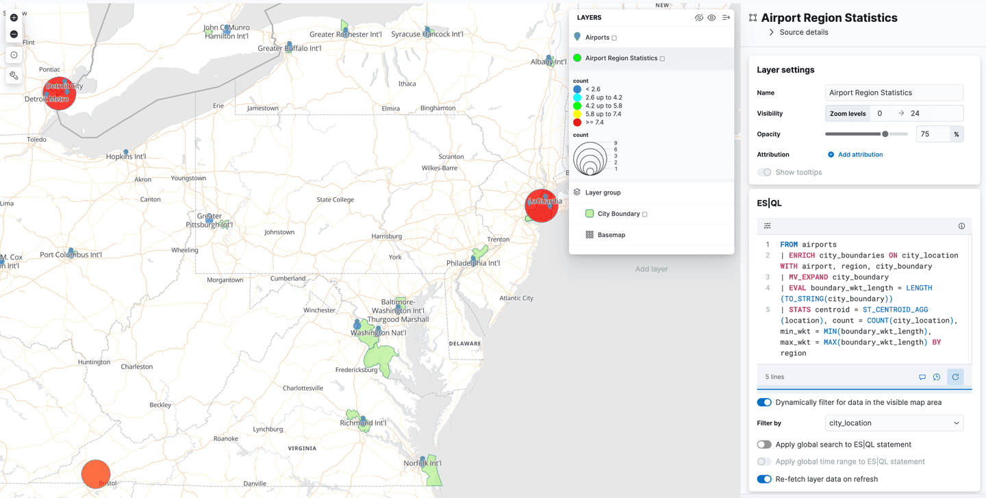
Kibana Maps
Kibana has added support for Spatial ES|QL in the Maps application. This means that you can now use ES|QL to search for geospatial data in Elasticsearch, and visualize the results on a map.
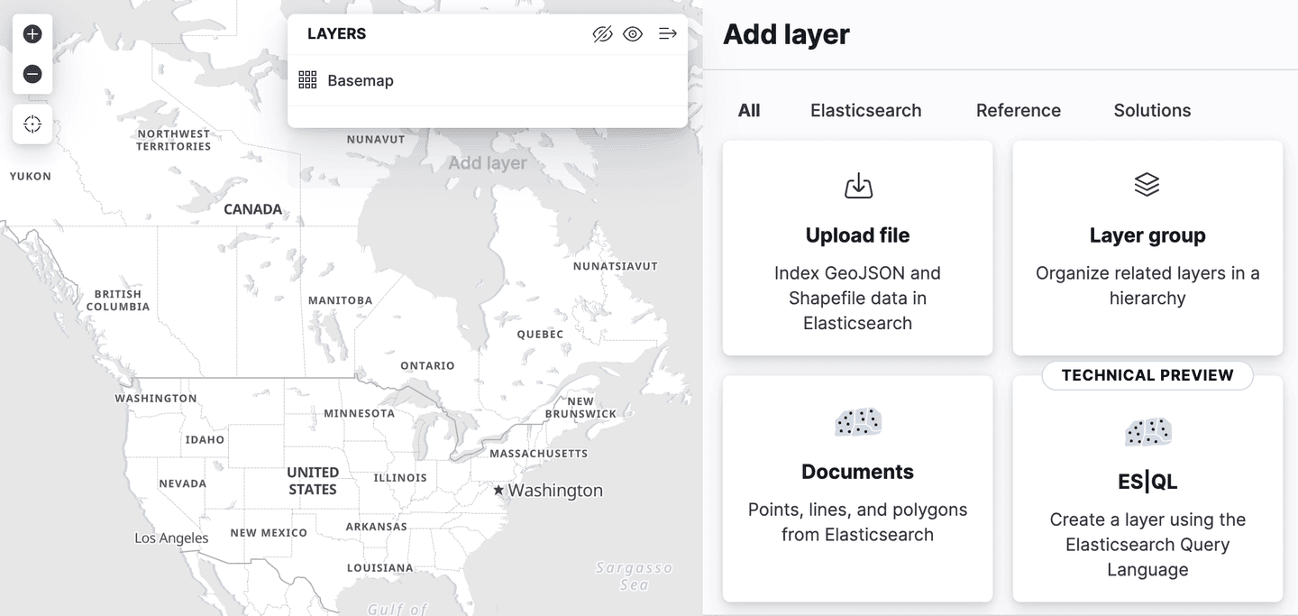
There is a new layer option in the add layers menu, called "ES|QL". Like all of the geospatial features described so far, this is in "technical preview". Selecting this option allows you to add a layer to the map based on the results of an ES|QL query. For example, you could add a layer to the map that shows all the airports in the world.
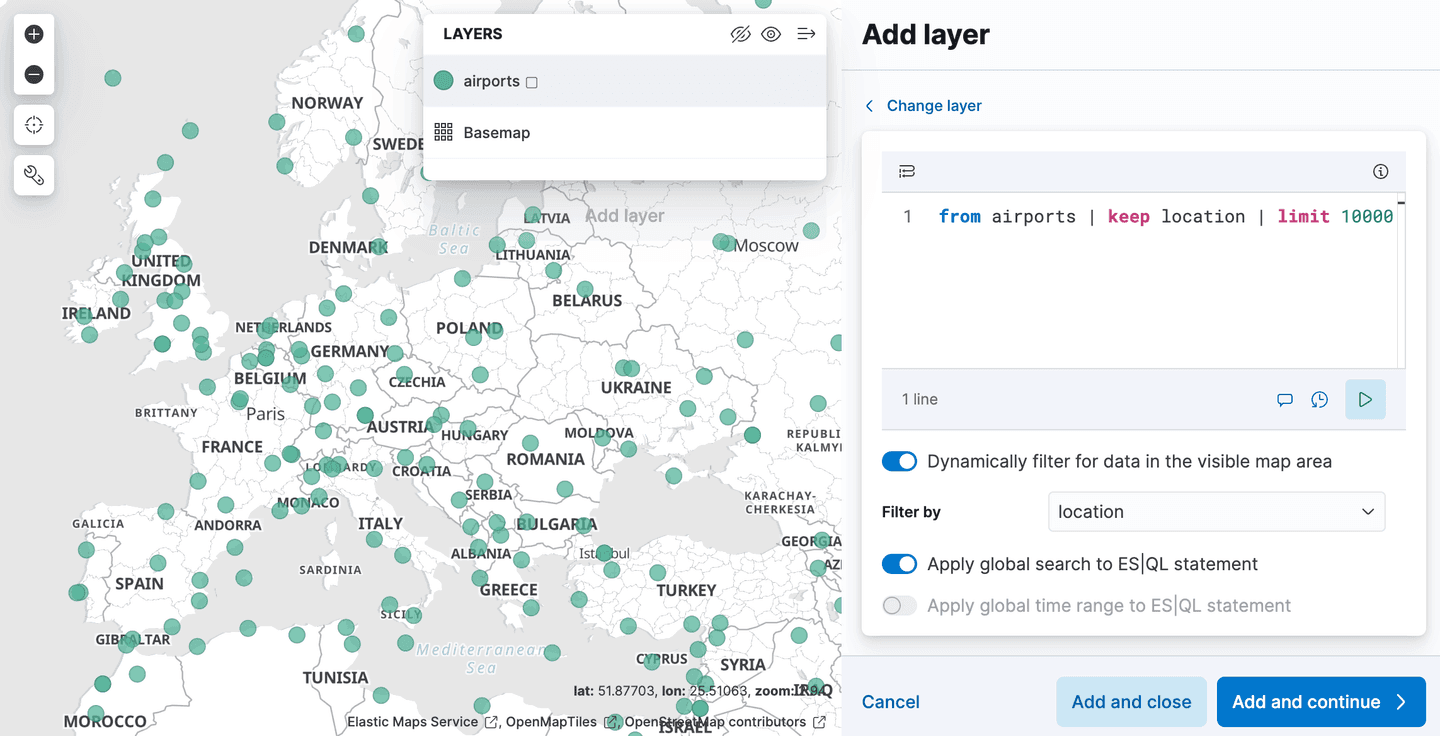
Or you could add a layer that shows the polygons from the airport_city_boundaries index, or even better, how about that complex ENRICH query above that generates statistics for how many airports are in each region?
What's next
You might have noticed in two of the examples above we squeezed in yet another spatial function ST_CENTROID_AGG. This is an aggregating function used in the STATS command, and the first of many spatial analytics features we plan to add to ES|QL. We'll blog about it when we've got more to show!
Before that, we want to tell you more about a particularly exciting feature we've worked on: the ability to perform spatial distance searches, one of the most used spatial search features of Elasticsearch. Can you imagine what the syntax for distance searches might look like? Perhaps similar to an OGC function? Stay tuned for the next blog in this series to find out!
Spoiler alert: Elasticsearch 8.15 has just been released, and spatial distance search with ES|QL is included!
Related Content

February 5, 2026
ES|QL dense vector search support
Using ES|QL for vector search on your dense_vector data.

January 19, 2026
Faster ES|QL stats with Swiss-style hash tables
How Swiss-inspired hashing and SIMD-friendly design deliver consistent, measurable speedups in Elasticsearch Query Language (ES|QL).

January 8, 2026
Hybrid search and multistage retrieval in ES|QL
Explore the multistage retrieval capabilities of ES|QL, using FORK and FUSE commands to integrate hybrid search with semantic reranking and native LLM completions.
December 12, 2025
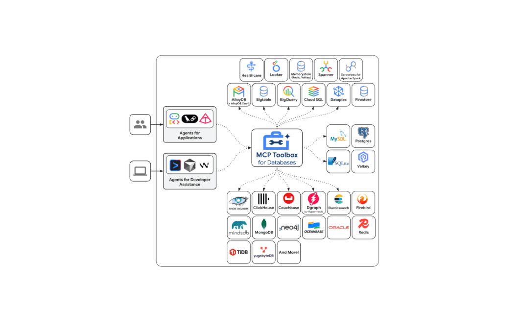
Introducing Elasticsearch support in the Google MCP Toolbox for Databases
Explore how Elasticsearch support is now available in the Google MCP Toolbox for Databases and leverage ES|QL tools to securely integrate your index with any MCP client.
December 2, 2025
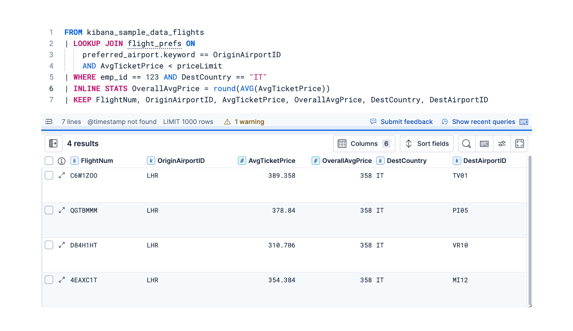
ES|QL in 9.2: Smart Lookup Joins and time-series support
Explore three separate updates to ES|QL in Elasticsearch 9.2: an enhanced LOOKUP JOIN for more expressive data correlation, the new TS command for time-series analysis, and the flexible INLINE STATS command for aggregation.