Using Kibana to ingest geospatial data into Elasticsearch for use in ES|QL

We recently published a blog describing how to use the new geospatial search features in ES|QL, Elasticsearch's new, powerful piped query language. To use these features, you need to have geospatial data in Elasticsearch. So in this blog, we'll show you how to ingest geospatial data, and how to use it in ES|QL queries.

Importing CSV data using Kibana

The data we used for the examples in the previous blog were based on data we use internally for integration tests. For your convenience we've, included it here in the form of a few CSV files that can easily be imported using Kibana. The data is a mix of airports, cities, and city boundaries. You can download the data from:

airports.csv
- This contains a merger of three datasets:
  - Airports (names, locations and related data) from Natural Earth
  - City locations from SimpleMaps
  - Airport elevations from The global airport database
airport_city_boundaries.csv
- This contains a merger of airport and city names from above with one new source:
  - City boundaries from OpenStreetMap

As you can guess, we spent some time combining these data sources into the two files above, with the goal of being able to test the geospatial features of ES|QL. This might not be quite the same as your specific data needs, but hopefully this gives you an idea of what is possible. In particular we want to demonstrate a few interesting things:

Importing data with geospatial fields together with other indexable data
Importing both geo_point and geo_shape data and using them together in queries
Importing data into two indexes that can be joined using a spatial relationship
Creating an ingest pipeline for facilitating future imports (beyond Kibana)
Some examples of ingest processors, like csv, convert and split

While we'll be discussing working with CSV data in this blog, it is important to understand there are several ways to add geo data using Kibana. Within the Map application you can upload delimited data like CSV, GeoJSON and ESRI ShapeFiles and you can also draw shapes directly in the Map. For this blog we'll focus on importing CSV files from the Kibana home page.

Importing the airports

The first file, airports.csv, has some interesting quirks we need to deal with. Firstly the columns have additional whitespace separating them, not typical of CSV files. Secondly, the type field is a multi-value field, which we need to split into separate fields. Finally, some fields are not strings, and need to be converted to the right type. All this can be done using Kibana's CSV import facility.

Start at the Kibana home-page. There is a section called "Get started by adding integrations", which has a link called "Upload a file":

Click on this link, and you will be taken to the "Upload file" page. Here you can drag and drop the airports.csv file, and Kibana will analyse the file and present you with a preview of the data. It should have automatically detected the delimiter as a comma, and the first row as the header row. However, it probably did not trim the extra whitespace between the columns, nor determined the types of the fields, assuming all fields are either text or keyword. We need to fix this.

Click Override settings and check the checkbox for Should trim fields, and Apply to close the settings. Now we need to fix the types of the fields. This is available on the next page, so go ahead and click Import.

First choose an index name, and then select Advanced to get to the field mappings and ingest processor page.

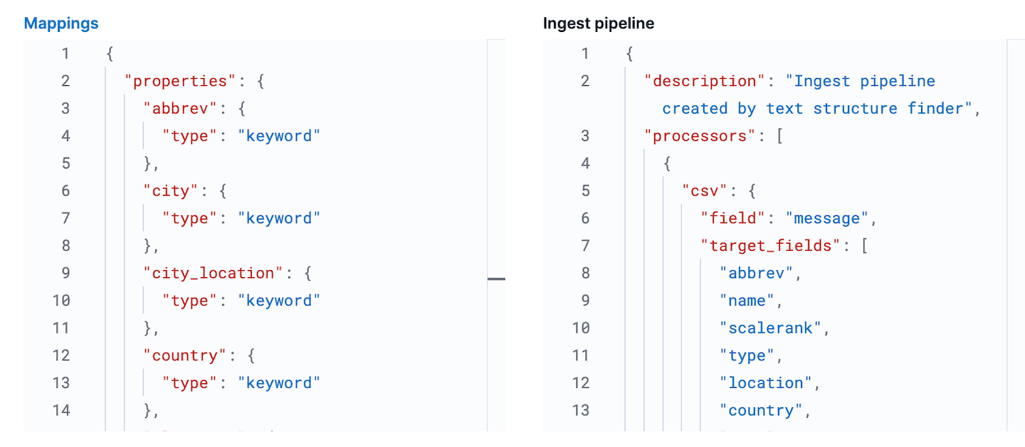
Here we need to make changes to both the field mappings for the index, as well as the ingest pipeline for importing the data. Firstly, while Kibana likely auto-detected the scalerank field as long, it mistakenly perceived the location and city_location fields as keyword. Edit them to geo_point, ending up with mappings that look something like:

{
  "properties": {
    "abbrev":        { "type": "keyword" },
    "city":          { "type": "keyword" },
    "city_location": { "type": "geo_point" },
    "country":       { "type": "keyword" },
    "elevation":     { "type": "double" },
    "location":      { "type": "geo_point" },
    "name":          { "type": "text" },
    "scalerank":     { "type": "long" },
    "type":          { "type": "keyword" }
  }
}

You have some flexibility here, but note that what type you choose will affect how the field is indexed and what kind of queries are possible. For example, if you leave location as keyword you cannot perform any geospatial search queries on it. Similarly, if you leave elevation as text you cannot perform numerical range queries on it.

Now it's time to fix the ingest pipeline. If Kibana auto-detected scalerank as long above, it will also have added a processor to convert the field to a long. We need to add a similar processor for the elevation field, this time converting it to double. Edit the pipeline to ensure you have this conversion in place. Before saving this, we want one more conversion, to split the type field into multiple fields. Add a split processor to the pipeline, with the following configuration:

{
  "split": {
    "field": "type",
    "separator": ":",
    "ignore_missing": true
  }
}

The final ingest pipeline should look like:

{
  "description": "Ingest pipeline created by text structure finder",
  "processors": [
    {
      "csv": {
        "field": "message",
        "target_fields": [
          "abbrev",
          "name",
          "scalerank",
          "type",
          "location",
          "country",
          "city",
          "city_location",
          "elevation"
        ],
        "ignore_missing": false,
        "trim": true
      }
    },
    {
      "convert": {
        "field": "scalerank",
        "type": "long",
        "ignore_missing": true
      }
    },
    {
      "convert": {
        "field": "elevation",
        "type": "double",
        "ignore_missing": true
      }
    },
    {
      "split": {
        "field": "type",
        "separator": ":",
        "ignore_missing": true
      }
    },
    {
      "remove": {
        "field": "message"
      }
    }
  ]
}

Note that we did not add a convert processor for the location and city_location fields. This is because the geo_point type in the field mapping already understands the WKT format of the data in these fields. The geo_point type can understand a range of formats, including WKT, GeoJSON, and more. If we had, for example, two columns in the CSV file for latitude and longitude, we would have needed to add either a script or a set processor to combine these into a single geo_point field (eg. "set": {"field": "location", "value": "{{lat}},{{lon}}"}).

We are now ready to import the file. Click Import and the data will be imported into the index with the mappings and ingest pipeline we just defined. If there are any errors ingesting the data, Kibana will report them here, so you can either edit the source data or the ingest pipeline and try again.

Notice that a new ingest-pipeline has been created. This can be viewed by going to the Stack Management section of Kibana, and selecting Ingest pipelines. Here you can see the pipeline we just created, and edit it if necessary. In fact the Ingest pipelines section can be used for creating and testing ingest pipelines, a very useful feature if you plan to do even more complex ingests.

If you want to explore this data immediately skip down to the later sections, but if you want to import the city boundaries as well, continue reading.

Importing the city boundaries

The city boundaries file available at airport_city_boundaries.csv is a bit simpler to import than the previous example. It contains a city_boundary field that is a WKT representation of the city boundary as a POLYGON, and a city_location field that is a geo_point representation of the city location. We can import this data in a similar way to the airports data, but with a few differences:

We needed to select the override setting Has header row since that was not autodetected
We did not need to trim fields, as the data was already clean of extra whitespace
We did not need to edit the ingest pipeline because all types were either string or spatial types
We did, however, have to edit the field mappings to set the city_boundary field to geo_shape and the city_location field to geo_point

Our final field mappings looked like:

{
  "properties": {
    "abbrev":        { "type": "keyword" },
    "airport":       { "type": "keyword" },
    "city":          { "type": "keyword" },
    "city_boundary": { "type": "geo_shape" },
    "city_location": { "type": "geo_point" },
    "region":        { "type": "text" }
  }
}

As with the airports.csv import before, simply click Import to import the data into the index. The data will be imported with the mappings we edited and ingest pipeline that Kibana defined.

Exploring the data with dev-tools

In Kibana it is usual to explore the indexed data with "Discover". However, if your intention is to write your own app using ES|QL queries, it might be more interesting to try access the raw Elasticsearch API. Kibana has a convenient console for experimenting with writing queries. This is called the Dev Tools console, and can be found in the Kibana side-bar. This console talks directly to the Elasticsearch cluster, and can be used to run queries, create indexes, and more.

Try the following:

POST /_query?error_trace=true&format=txt
{
  "query": """
FROM airports
| EVAL distance = ST_DISTANCE(city_location, TO_GEOPOINT("POINT(12.565 55.673)"))
| WHERE distance < 1000000 AND scalerank < 6 AND distance > 10000
| SORT distance ASC
| KEEP distance, abbrev, name, location, country, city, elevation
| LIMIT 10
  """
}

This should provide the following results:

distance	abbrev	name	location	country	city	elevation
273418.05776847183	HAM	Hamburg	POINT (10.005647830925 53.6320011640866)	Germany	Norderstedt	17.0
337534.653466062	TXL	Berlin-Tegel Int'l	POINT (13.2903090925074 52.5544287044101)	Germany	Hohen Neuendorf	38.0
483713.15032266214	OSL	Oslo Gardermoen	POINT (11.0991032762581 60.1935783171386)	Norway	Oslo	208.0
522538.03148094116	BMA	Bromma	POINT (17.9456175406145 59.3555902065112)	Sweden	Stockholm	15.0
522538.03148094116	ARN	Arlanda	POINT (17.9307299016916 59.6511203397372)	Sweden	Stockholm	38.0
624274.8274399083	DUS	Düsseldorf Int'l	POINT (6.76494446612174 51.2781820420774)	Germany	Düsseldorf	45.0
633388.6966435644	PRG	Ruzyn	POINT (14.2674849854076 50.1076511703671)	Czechia	Prague	381.0
635911.1873311149	AMS	Schiphol	POINT (4.76437693232812 52.3089323889822)	Netherlands	Hoofddorp	-3.0
670864.137958866	FRA	Frankfurt Int'l	POINT (8.57182286907608 50.0506770895207)	Germany	Frankfurt	111.0
683239.2529970079	WAW	Okecie Int'l	POINT (20.9727263383587 52.171026749259)	Poland	Piaseczno	111.0

Visualizing the data with Maps

Kibana Maps is a powerful tool for visualizing geospatial data. It can be used to create maps with multiple layers, each layer representing a different dataset. The data can be filtered, aggregated, and styled in various ways. In this section, we will show you how to create a map in Kibana Maps using the data we imported in the previous section.

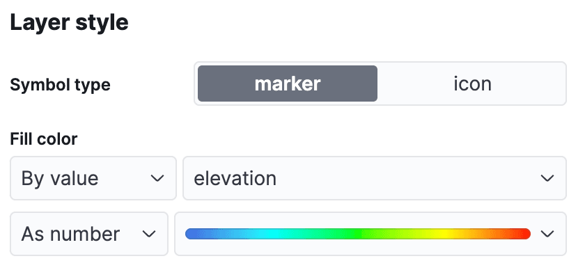
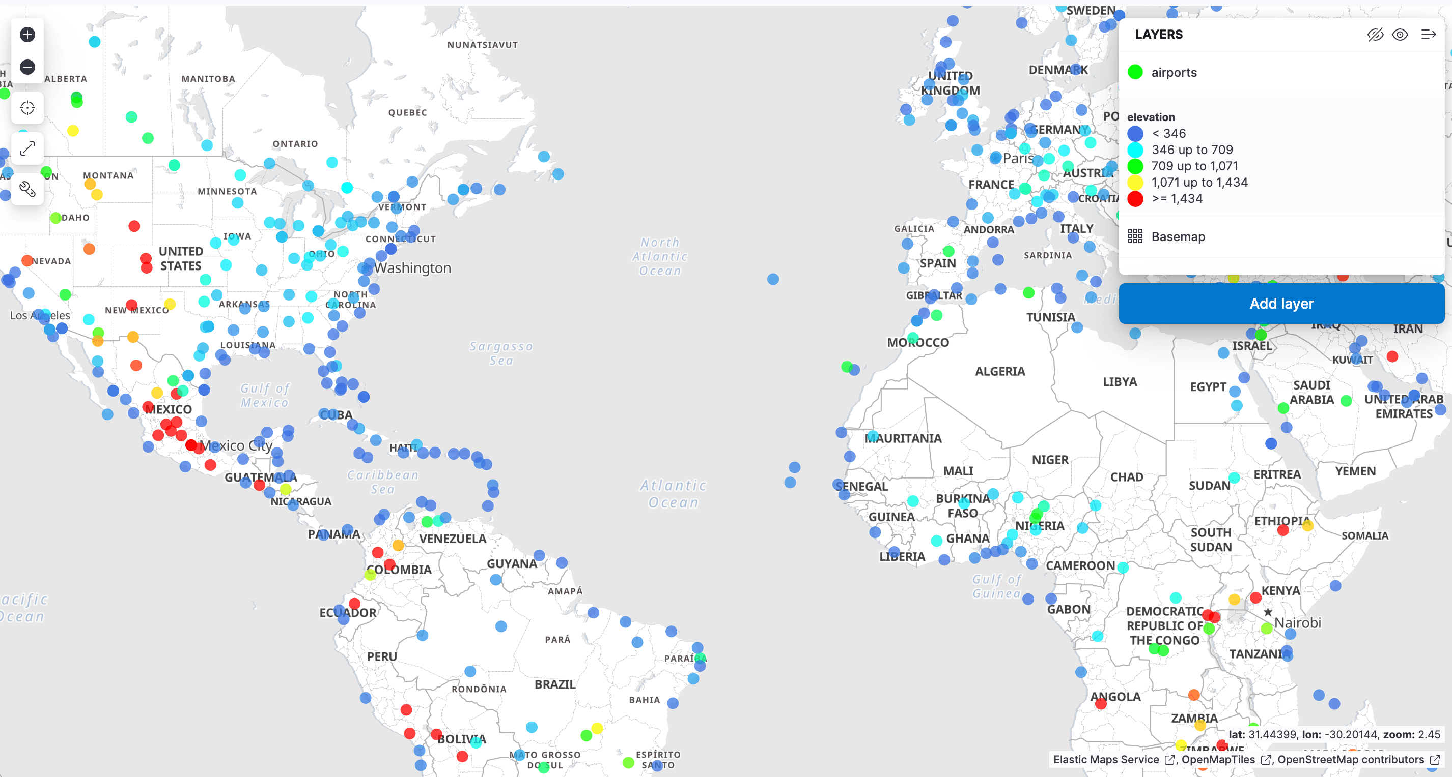
In the Kibana menu, navigate to Analytics->Maps to open a new map view. Click on Add Layer and select Documents, choosing the data view airports and then editing the layer style to color the markers using the elevation field, so we can easily see how high each airport is.

Click 'Keep changes' to save the Map:

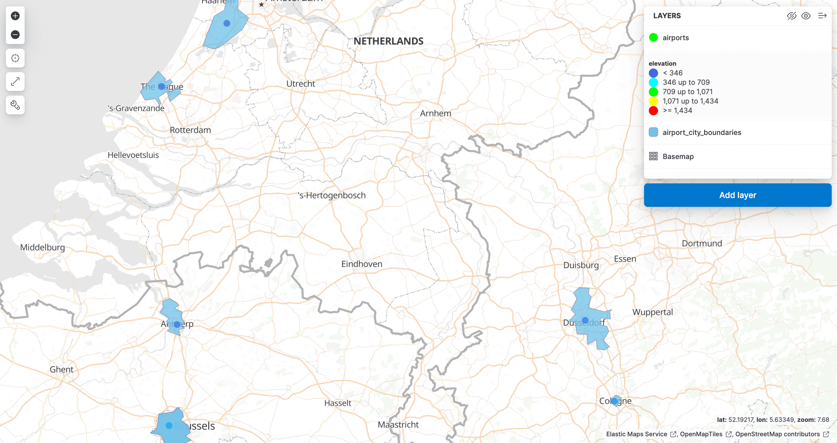
Now add a second layer, this time selecting the airport_city_boundaries data view. This time, we will use the city_boundary field to style the layer, and set the fill color to a light blue. This will show the city boundaries on the map. Make sure to reorder the layers to ensure that the airport markers are on top.

Kibana Maps - City Boundaries Layer Style

Spatial joins

ES|QL does not support JOIN commands, but you can achieve a special case of a join using the ENRICH command. This command operates akin to a 'left join' in SQL, allowing you to enrich results from one index with data from another index based on a spatial relationship between the two datasets.

For example, let's enrich the results from a table of airports with additional information about the city they serve by finding the city boundary that contains the airport location, and then perform some statistics on the results:

FROM airports
| ENRICH city_boundaries ON city_location WITH airport, region, city_boundary
| STATS
    centroid = ST_CENTROID_AGG(location),
    count = COUNT(city_location)
    BY region
| SORT count DESC
| LIMIT 10

If you run this query without first preparing the enrich index, you will get an error message like:

cannot find enrich policy [city_boundaries]

This is because, as we mentioned before, ES|QL does not support true JOIN commands. One important reason for this is that Elasticsearch is a distributed system, and joins are expensive operations that can be difficult to scale. However, the ENRICH command can be quite efficient, because it makes use of specially prepared enrich indexes that are duplicated across the cluster, enabling local joins to be performed on each node.

To better understand this, let's focus on the ENRICH command in the query above:

FROM airports
| ENRICH city_boundaries ON city_location WITH airport, region, city_boundary

This command instructs Elasticsearch to enrich the results retrieved from the airports index, and perform an intersects join between the city_location field of the original index, and the city_boundary field of the airport_city_boundaries index, which we used in a few examples earlier. But some of this information is not clearly visible in this query. What we do see is the name of an enrich policy city_boundaries, and the missing information is encapsulated within that policy definition.

{
  "geo_match": {
    "indices": "airport_city_boundaries",
    "match_field": "city_boundary",
    "enrich_fields": ["city", "airport", "region", "city_boundary"]
  }
}

Here we can see that it will perform a geo_match query (intersects is the default), the field to match against is city_boundary, and the enrich_fields are the fields we want to add to the original document. One of those fields, the region was actually used as the grouping key for the STATS command, something we could not have done without this 'left join' capability. For more information on enrich policies, see the enrich documentation.

The enrich indexes and policies in Elasticsearch were originally designed for enriching data at index time, using data from another prepared enrich index. In ES|QL, however, the ENRICH command works at query time, and does not require the use of ingest pipelines. This effectively makes it quite similar to an SQL LEFT JOIN, except youn cannot join any two indexes, only a normal index on the left with a specially prepared enrich index on the right.

In either case, whether for ingest pipelines or use in ES|QL, it is necessary to perform a few preparatory steps to set up the enrich index and policy. We already imported the airport_city_boundaries index above, but this is not directly usable as an enrich index in the ENRICH command. We first need to perform two steps:

Create the enrich policy described above to define the source index, the field in the source index to match against, and the fields to return once matched.
Execute this policy to create the enrich index. This will build a special internal index, by reading the original source index into a more efficient data structure which is copied across the cluster.

The enrich policy can be created using the following command:

PUT /_enrich/policy/city_boundaries
{
  "match": {
    "indices": "airport_city_boundaries",
    "match_field": "city_boundary",
    "enrich_fields": ["city", "airport", "region", "city_boundary"]
  }
}

And the policy can be executed using the following command:

POST /_enrich/policy/city_boundaries/_execute

Note that if you ever change the contents of the airport_city_boundaries index, you will need to re-execute this policy to see the changes reflected in the enrich index. Now let's run the original ES|QL query again:

FROM airports
| ENRICH city_boundaries ON city_location WITH airport, region, city_boundary
| STATS
    centroid = ST_CENTROID_AGG(location),
    count = COUNT(city_location)
    BY region
| SORT count DESC
| LIMIT 10

This returns the top 5 regions with the most airports, along with the centroid of all the airports that have matching regions, and the range in length of the WKT representation of the city boundaries within those regions:

centroid	count	region
POINT (-12.139086859300733 31.024386116624648)	126	null
POINT (-83.10398317873478 42.300230911932886)	3	Detroit
POINT (39.74537850357592 47.21613017376512)	3	городской округ Батайск
POINT (-156.80986787192523 20.476673701778054)	3	Hawaii
POINT (-73.94515332765877 40.70366442203522)	3	City of New York
POINT (-83.10398317873478 42.300230911932886)	3	Detroit
POINT (-76.66873019188643 24.306286952923983)	2	New Providence
POINT (-3.0252167768776417 51.39245774131268)	2	Cardiff
POINT (-115.40993484668434 32.73126147687435)	2	Municipio de Mexicali
POINT (41.790108773857355 50.302146775648)	2	Центральный район
POINT (-73.88902732171118 45.57078813901171)	2	Montréal

You may also notice that the most commonly found region was null. What could this imply? Recall that I likened this command to a 'left join' in SQL, meaning if no matching city boundary is found for an airport, the airport is still returned but with null values for the fields from the airport_city_boundaries index. It turns out there were 125 airports that found no matching city_boundary, and one airport with a match where the region field was null. This lead to a count of 126 airports with no region in the results. If your use case requires that all airports can be matched to a city boundary, that would require sourcing additional data to fill in the gaps. It would be necessary to determine two things:

which records in the airport_city_boundaries index do not have city_boundary fields
which records in the airports index do not match using the ENRICH command (ie. do not intersect)

ES|QL in Kibana Maps

Kibana has added support for Spatial ES|QL in the Maps application. This means that you can now use ES|QL to search for geospatial data in Elasticsearch, and visualize the results on a map.

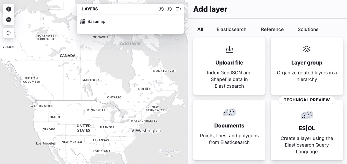
There is a new layer option in the add layers menu, called "ES|QL". Like all of the geospatial features described so far, this is in "technical preview". Selecting this option allows you to add a layer to the map based on the results of an ES|QL query. For example, you could add a layer to the map that shows all the airports in the world.

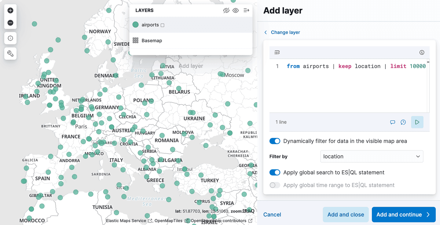
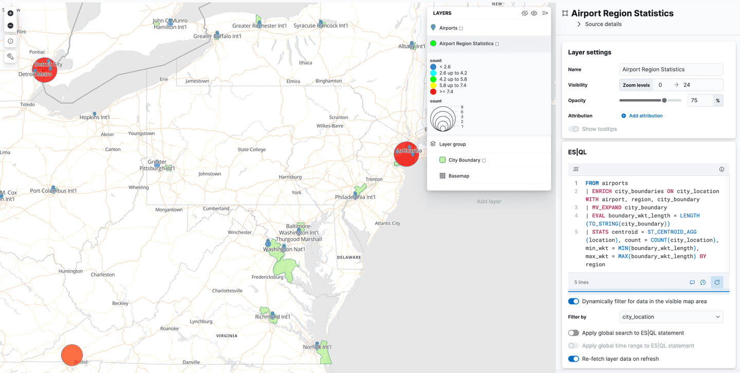
Or you could add a layer that shows the polygons from the airport_city_boundaries index, or even better, how about that complex ENRICH query above that generates statistics for how many airports are in each region?

What's next

The previous Geospatial search blog focused on the use of functions like ST_INTERSECTS to perform searching, available in Elasticsearch since 8.14. And this blog shows you how to import the data we used for those searches. However, Elasticsearch 8.15 came with a particularly interesting function: ST_DISTANCE which can be used to perform efficient spatial distance searches, and this will be the topic of the next blog!

Want to get Elastic certified? Find out when the next Elasticsearch Engineer training is running!

Elasticsearch is packed with new features to help you build the best search solutions for your use case. Dive into our sample notebooks to learn more, start a free cloud trial, or try Elastic on your local machine now.