Observe, protect, and search your data with a single solution. From application monitoring to threat detection, Kibana is your versatile platform for critical use cases. Start your free 14-day trial now.
To explain the fundamentals of building Vega visualizations in Kibana I'll use 2 examples, present in this GitHub repo. Specifically, I'll cover:
- Data sourcing with Elasticsearch aggregations
- Axes and marks
- Events and signals such as tooltips and updating the central Kibana dashboard filters
I'll also share some useful tips for debugging issues in visualization along the way.
About Kibana and Vega
Kibana allows you to build many common visualization types such as column and bar charts, heatmaps, and even metric cards quickly. As a frontend engineer, low-code tools for building visualizations are great not only for prototyping but also for allowing users to potentially build their own basic charts so I can focus on more complex visualizations.
Vega and Vega-Lite are related grammars for building visualizations and graphics in a JSON format. Both can be used in Kibana for building complex visualizations to be included in Kibana dashboards. Yet they have a steep learning curve making it difficult to write and debug issues in your syntax.
Why Vega?
Vega and Vega-Lite are related grammars for loading and transforming data to build graphics and visualizations in a JSON format. Vega-Lite is a more concise syntax that is converted to Vega prior to rendering. So for those new to Vega I would recommend starting with Vega-Lite first for this reason.
Since Kibana provides many drag-and-drop tools such as Lens and TSVB for creating charts on top of Elasticsearch data, Vega should be used in the following circumstances:
- The visualization type you need is not available via other editors. Key examples would be those wanting to create Chord or Radar diagrams that are not available in Lens.
- An existing visualization does not support or lacks a given feature that you need.
- Create visualizations that require complex calculations or nested aggregation structures.
- You need to create charts based on data that meet the challenges discussed in the Kibana Vega documentation.
- The visualization you need to create does not rely on tables or conditional queries.
Pre-requisites
Leveraging the Sample flight data dataset available in Elastic Cloud, we shall build 2 new visualizations:
- A cancellation summary showing the logo and number of cancellations for each airline over the selected time period.
- A radar chart showing the number of flights for each carrier to key destinations.
Before building these visualizations, please ensure you have completed the following steps:
- Create an Elastic Cloud cluster, either by starting a free trial or using your existing cluster.
- Add the Sample flight data dataset using the Add the sample data instructions in the documentation.
These examples use Kibana v8.14 and Vega-Lite v5.2.0. These versions are available by default in Kibana without the need for additional installation.
Basic Anatomy of a Vega Visualization
Creating your first visualization in Vega is possible from various places in Kibana, including the Visualize Library and a dashboard. Irrespective of where you are, select the Custom Visualization:

The sample Vega specification is written in HJSON. This JSON extension supports comments, multi-line strings and other useful language features such as the removal of quotes and commas for readability. For any Vega or Vega-Lite visualization you write in Kibana, you will need these elements:
- $schema: the language specification for the version of Vega or Vega-Lite that your visualization is written in. Our examples use the default schema for v5.x of Vega-Lite.
- title to denote the visualization title. Alternatively, another metadata field that could be useful in describing your visualization is description.
- data: the Elasticsearch query and related settings used to pull data from Elasticsearch for use in your chart.
- At least one attribute from mark, marks or layer to define the graphical elements to show individual data points and line series.
- encoding attributes that contain the visual properties and corresponding data values that mark elements need for rendering. Typical examples include fill, color and text positions but there are many different types.
Other elements used are covered via the examples in subsequent sections.
Example 1: Summary with images
Our first visualization is a simple summary widget, written using Vega-Lite, containing text and image data points:

If you want to dive straight into the code, the full solution is available here.
Schema
We must ensure the $schema attribute points to the Vega-Lite correct schema to prevent confusing errors:
Data source
Our simple infographic will show the number of cancellations by airline within the selected timeframe. In simple Elasticsearch Query DSL we would trigger the following request to get these results:
In any Vega or Vega-Lite visualization, the data attribute defines the source of data to be visualized. In Kibana, we tend to pull data from an Elasticsearch index. Instead of a string for the url value, data.url can be used as a custom Kibana-specific object treated as a context-aware Elasticsearch query, which provides additional filter context from dashboard elements such as the filter bar and date picker. The Elasticsearch query is specified in the body of the data.url object.
As covered in the documentation, there are several special tokens that Kibana parses for and considers when fetching data to pass to the Vega renderer. In this example, we pass a query making use of the %dashboard_context-must_clause% and %timefilter% characters to query for canceled flights in the kibana_sample_data_flights index within the timeframe selected in the dashboard time filter control, before aggregating the results using a terms aggregation.
You may wonder what the format property does. Running our initial query in the DevTools console, you'll see the results of interest are present in the field aggregations.carriers.buckets:
The format property discards the additional contents of the response, leaving us with the clean key-value pairs in source_0 which is the default name for the data source object. The resulting data is visible within the Kibana Vega Debug option under the Inspector:

Text Elements
The next step is to show the airline, denoted by the key field, and the number of cancellations using doc_count from the source data. Simple Vega-Lite visualizations use a single mark attribute. However, if you need to have multiple layers in your visualization the layer attribute allows you to specify several mark types, as shown below:
The above example shows 2 text marks presenting the carrier and number of cancellations, with the latter encoding element adding a color series based on the key attribute in the data series. However, running the above shows all elements overlap:

If your visualization is blank try expanding the time range.
Adding an invisible x-axis to the encoding attribute in this situation can separate the values based on the key:
The result is the below-color-coded cancellation counts by airline:

Images
Now add the image elements for each carrier. Vega-Lite has support for adding images for each data point using the image mark.
Enriching each data point with the image URL is possible using different types of transformations using the transform attribute. Here we add the URL for each image according to the value of the key attribute of each record, as denoted by the datum prefix, and store it in the new field img:
In the Kibana inspector, the new data_0 field contains the image URL based on the defined mapping:

This URL can be used in an image mark added to the collection of layers:
You may be surprised at this point to see the following error message instead of the images:
External URLs are not enabled. Add vis_type_vega.enableExternalUrls: true to kibana.yml
By default, Kibana blocks external URLs. Once setting vis_type_vega.enableExternalUrls: true is added to your kibana.yml file, AKA the user settings on the Kibana instance in your cloud configuration, the images will be visible:
Autosizing
When it comes to adding this component to your dashboards, resizing is important given the horizontal spread of this control. By default, Vega-Lite does not recalculate layouts on each view change. To configure the auto-fitting and resize options, the below auto-sizing configuration needs to be added to the top-level specification:
When using the fit sizing type be aware of the view requirements set out in the Vega-Lite documentation. Check out the GitHub repo for the full visualization code.
Example 2: Radar Chart
Our second visualization is a Radar or Spider chart, which is great for plotting a series of values across multiple categories. Our example, written in Vega, shows the number of flights to each destination by carrier:

This solution is based on the radar chart example in the Vega documentation. The data sourcing, marks, tooltips and click event code are discussed in subsequent sections. The full code is available here.
Schema
As Kibana supports Vega and Vega-Lite, we need to ensure the $schema attribute points to the correct schema to prevent confusing errors. As our example used the Vega-Lite schema before, ensure you set $schema to the appropriate Vega schema:
Data source
Our data source is a simple multi-terms aggregation to get the total number of flights by the destination and carrier combination:
The aggregate provides a composite key and document count within the result object aggregations.destinations_and_carrier.buckets similar to the following:
The data attribute accepts the filter context and timestamp from the dashboard controls using the custom %context% and %timefield% tags that Kibana replaces before passing to the Vega renderer:
Notice that we are not using a query in our Elasticsearch request to filter the data here. You cannot use query and the %context% and %timefield% combination in the same data source. If you require filtering alongside time filtering based on the dashboard selection, please pass both as covered above in example 1.
Once we have our results from Elasticsearch, we can create a flattened data source table pulling out the array elements using a formula expression, normalizing missing values using the impute transform, and an aggregated structure keys containing the destinations for the outer web of the chart using transformations. As you'll see below we use the source attribute to define the Elasticsearch aggregation source that we aptly named source in the previous step:
With the above transforms our additional sources look similar to the below:


Basic chart
To build a simple radar chart we require the available radius to draw the control, along with definitions of the scales and marks for each element.
The radius can be calculated based on the width using a signal. Signals in both Vega and Vega-Lite are dynamic variables storing values that can drive interactive behaviors and updates. Typical examples include updates based on mouse events or the panel width. Here we specify a signal to calculate the radius of the chart based on the canvas width:
Looking at the desired visualization, you'll see we need to map values for the radial access on the outside, as well as elements inside the chart. This is where scales come in handy. These scales are used by the marks to render the visual elements in the correct place relative to others on the scale:
The scale property allows us to define the positions for the elements on the lines of our radar chart via a linear scale, the range of positions for the outside destinations using a point scale and also the color scheme for the filled carrier segments in the middle of our visualization.

As illustrated in the above-annotated chart, our radar chart contains several different types of marks:
- The shaded polygons for each airline, are denoted by the line named
category-line. - Text labels for each destination, aptly named
value-text. - Diagonal lines running from the edge to the center, known as series
radial-grid. This series makes use of theangularscale discussed previously along with therulemark as opposed to thelinemark. - The series
key-labeldescribes the destination labels running on the outside of the chart. - Lastly, the line running along the outside of the radar chart is known as the line mark
outer-line.
The full code for these marks is the following:
At this point, a basic chart will be visible. Note that depending on whether dark or light mode is enabled in Kibana, some text elements may not be visible. Currently, it is impossible to obtain the selected theme information for Kibana in Vega (but is proposed in issue #178254), so try to stick to category color schemes and colors visible in both schemes where possible.
Legend
Adding a legend to this chart is important to communicate which color represents which carrier. Legends can be defined within various scopes of the specification. In our case, the easiest way is to define the legend as a top-level attribute, specifying the fill option to use our color scale:
Tooltips
Tooltips are another utility that makes scrutinizing individual values in busy charts easier. They also provide additional context to an individual data point. In our case, it shows the destination and carrier alongside the number of flights. Much like legends, they can be specified at several different places in our specification.
Firstly, we need to update the datum object with the data point value over which the user hovers. You can achieve this using the update option on mouseover and mouseout events, as highlighted in the below snippet:
The main configuration for the tooltip is then applied to the mark upon which we want to trigger showing the tooltip when the mouse is over that particular element. In our case, this is the mark named value-text defined previously:
Notice that the data points are stored in a separate datum object under the generic datum element that forms the context of the data point. This is why we have two occurrences within the path.
Finally, we have the completed chart that we're looking for!
Updating global dashboard state
Upon adding these visualizations to our flight dashboard, you'll notice that clicking on data points on Lens and TSVB-created controls updates the global dashboard filters, but that our Vega and Vega-Lite controls do not:

By default, click events are not passed to the dashboard filter, and need to be added using additional signals. Kibana provides an extended set of functions to trigger a data update and change the dashboard query and date-time filters.
For example, to add the selected carrier to the global dashboard filter, add a click event handler to the value-text mark to add the value for the airline using the kibanaAddFilter function:
The result is that all applicable charts will filter their results to show the carrier selected when we click the radar chart element:

In this example, users can only select a single airline. But if handling updates or removals of filter events is needed specifically, all filters can be removed using the kibanaremoveFilter and kibanaRemoveAllFilters functions.
For the final version of this visualization, check out the GitHub repo.
Debugging tips
Even with the best copy-pasting skills, every developer runs into errors when trying to adapt these examples, and the central Vega and Vega-Lite examples, to their dataset. For this reason, being familiar with common errors and inspection tools is vital.
Kibana provides the inspector, which we have seen used in various parts of this blog, which allows you to look at the Elasticsearch request and response structure, as well as data values and signals in your visualization:


For those more at home with the browser developer tools, the VEGA_DEBUG object is exposed via the Kibana Vega plugin in the console:

As you'll see in the above screenshot of Chrome DevTools, the debugging expressions covered in the Vega debugging guide are accessible through VEGA_DEBUG. For example, inspecting the values of the radius signal in our radar chart using view.signal(signal_name)is possible via VEGA_DEBUG.view.signal('radius').
Throughout researching this piece, I noted particular errors that you may encounter in your development:
- Cannot convert undefined or null to object is the equivalent of a NullPointerException in some languages. For using nested objects check the full path is available, especially when using the
formatattribute with the Elasticsearch query in thedataobject. A related warning is Cannot read properties of undefined - Infinite extent for field "field": [Infinity, -Infinity]: this is a common warning developers experience that relates to the set of values for the specified field. Check the values and data types using the inspector.
- Warning url dropped as it is incompatible with "text" is an example where an attribute is being used that is not compatible with a specific mark or should be specified in another place. For these issues check the language specification.
Some common questions and errors have already been asked in the community forums. Do search to see if your issue has been previously answered. Alternatively, raise a new issue that the community can try to help with.
Conclusion
While Lens and TSVB controls provide a variety of chart types for showcasing data, Vega and Vega-Lite are the recommended approaches for building advanced visualizations in Kibana. In this piece, the examples have covered essential techniques for visualizing data and updating the view in response to user actions such as clicks.
When building your own Vega visualization, try including these examples or others from the Vega and Vega Lite example pages in Kibana and adapting the query to use your data. Share your questions and visualizations with us in the community forums.
Happy visualizing!
Resources
Related Content

Improving Kibana dashboard interactivity with variable controls
Discover how to use variable controls in Kibana 8.18+ to filter individual visualizations, adjust time intervals, and group by different fields in Kibana dashboards.
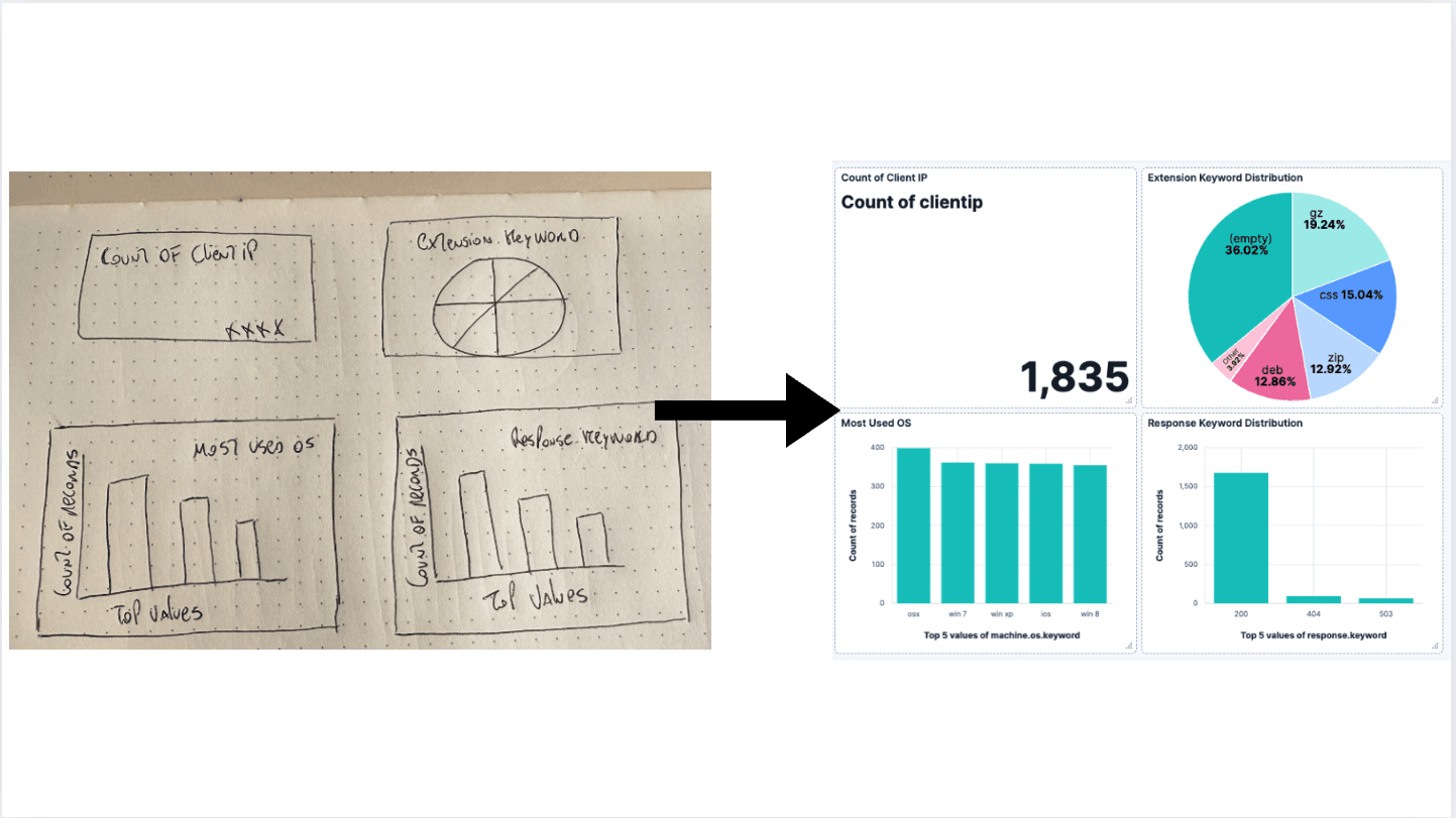
AI-powered dashboards: From a vision to Kibana
Generate a dashboard using an LLM to process an image and turn it into a Kibana Dashboard.

April 18, 2025
Kibana Alerting: Breaking past scalability limits & unlocking 50x scale
Kibana Alerting now scales 50x better, handling up to 160,000 rules per minute. Learn how key innovations in the task manager, smarter resource allocation, and performance optimizations have helped break past our limits and enabled significant efficiency gains.

March 3, 2025
Fast Kibana Dashboards
From 8.13 to 8.17, the wait time for data to appear on a dashboard has improved by up to 40%. These improvements are validated both in our synthetic benchmarking environment and from metrics collected in real user’s cloud environments.

Spotify Wrapped part 2: Data analysis and visualization
We will dive deeper into your Spotify data than ever before and explore connections you didn't even know existed.