- Elasticsearch Guide: other versions:
- Getting Started
- Setup
- Breaking changes
- API Conventions
- Document APIs
- Search APIs
- Search
- URI Search
- Request Body Search
- Search Template
- Search Shards API
- Aggregations
- Min Aggregation
- Max Aggregation
- Sum Aggregation
- Avg Aggregation
- Stats Aggregation
- Extended Stats Aggregation
- Value Count Aggregation
- Percentiles Aggregation
- Percentile Ranks Aggregation
- Cardinality Aggregation
- Geo Bounds Aggregation
- Top hits Aggregation
- Scripted Metric Aggregation
- Global Aggregation
- Filter Aggregation
- Filters Aggregation
- Missing Aggregation
- Nested Aggregation
- Reverse nested Aggregation
- Children Aggregation
- Terms Aggregation
- Significant Terms Aggregation
- Range Aggregation
- Date Range Aggregation
- IPv4 Range Aggregation
- Histogram Aggregation
- Date Histogram Aggregation
- Geo Distance Aggregation
- GeoHash grid Aggregation
- Facets
- Suggesters
- Multi Search API
- Count API
- Search Exists API
- Validate API
- Explain API
- Percolator
- More Like This API
- Indices APIs
- Create Index
- Delete Index
- Get Index
- Indices Exists
- Open / Close Index API
- Put Mapping
- Get Mapping
- Get Field Mapping
- Types Exists
- Delete Mapping
- Index Aliases
- Update Indices Settings
- Get Settings
- Analyze
- Index Templates
- Warmers
- Status
- Indices Stats
- Indices Segments
- Indices Recovery
- Clear Cache
- Flush
- Refresh
- Optimize
- Upgrade
- Shadow replica indices
- cat APIs
- Cluster APIs
- Query DSL
- Queries
- Match Query
- Multi Match Query
- Bool Query
- Boosting Query
- Common Terms Query
- Constant Score Query
- Dis Max Query
- Filtered Query
- Fuzzy Like This Query
- Fuzzy Like This Field Query
- Function Score Query
- Fuzzy Query
- GeoShape Query
- Has Child Query
- Has Parent Query
- Ids Query
- Indices Query
- Match All Query
- More Like This Query
- Nested Query
- Prefix Query
- Query String Query
- Simple Query String Query
- Range Query
- Regexp Query
- Span First Query
- Span Multi Term Query
- Span Near Query
- Span Not Query
- Span Or Query
- Span Term Query
- Term Query
- Terms Query
- Top Children Query
- Wildcard Query
- Minimum Should Match
- Multi Term Query Rewrite
- Template Query
- Filters
- And Filter
- Bool Filter
- Exists Filter
- Geo Bounding Box Filter
- Geo Distance Filter
- Geo Distance Range Filter
- Geo Polygon Filter
- GeoShape Filter
- Geohash Cell Filter
- Has Child Filter
- Has Parent Filter
- Ids Filter
- Indices Filter
- Limit Filter
- Match All Filter
- Missing Filter
- Nested Filter
- Not Filter
- Or Filter
- Prefix Filter
- Query Filter
- Range Filter
- Regexp Filter
- Script Filter
- Term Filter
- Terms Filter
- Type Filter
- Queries
- Mapping
- Analysis
- Analyzers
- Tokenizers
- Token Filters
- Standard Token Filter
- ASCII Folding Token Filter
- Length Token Filter
- Lowercase Token Filter
- Uppercase Token Filter
- NGram Token Filter
- Edge NGram Token Filter
- Porter Stem Token Filter
- Shingle Token Filter
- Stop Token Filter
- Word Delimiter Token Filter
- Stemmer Token Filter
- Stemmer Override Token Filter
- Keyword Marker Token Filter
- Keyword Repeat Token Filter
- KStem Token Filter
- Snowball Token Filter
- Phonetic Token Filter
- Synonym Token Filter
- Compound Word Token Filter
- Reverse Token Filter
- Elision Token Filter
- Truncate Token Filter
- Unique Token Filter
- Pattern Capture Token Filter
- Pattern Replace Token Filter
- Trim Token Filter
- Limit Token Count Token Filter
- Hunspell Token Filter
- Common Grams Token Filter
- Normalization Token Filter
- CJK Width Token Filter
- CJK Bigram Token Filter
- Delimited Payload Token Filter
- Keep Words Token Filter
- Keep Types Token Filter
- Classic Token Filter
- Apostrophe Token Filter
- Character Filters
- ICU Analysis Plugin
- Modules
- Index Modules
- Testing
- Glossary of terms
WARNING: Version 1.5 of Elasticsearch has passed its EOL date.
This documentation is no longer being maintained and may be removed. If you are running this version, we strongly advise you to upgrade. For the latest information, see the current release documentation.
Percentiles Aggregation
editPercentiles Aggregation
editA multi-value metrics aggregation that calculates one or more percentiles
over numeric values extracted from the aggregated documents. These values
can be extracted either from specific numeric fields in the documents, or
be generated by a provided script.
This functionality is in technical preview and may be changed or removed in a future release. Elastic will work to fix any issues, but features in technical preview are not subject to the support SLA of official GA features.
Percentiles show the point at which a certain percentage of observed values occur. For example, the 95th percentile is the value which is greater than 95% of the observed values.
Percentiles are often used to find outliers. In normal distributions, the 0.13th and 99.87th percentiles represents three standard deviations from the mean. Any data which falls outside three standard deviations is often considered an anomaly.
When a range of percentiles are retrieved, they can be used to estimate the data distribution and determine if the data is skewed, bimodal, etc.
Assume your data consists of website load times. The average and median load times are not overly useful to an administrator. The max may be interesting, but it can be easily skewed by a single slow response.
Let’s look at a range of percentiles representing load time:
By default, the percentile metric will generate a range of
percentiles: [ 1, 5, 25, 50, 75, 95, 99 ]. The response will look like this:
{
    ...

   "aggregations": {
      "load_time_outlier": {
         "values" : {
            "1.0": 15,
            "5.0": 20,
            "25.0": 23,
            "50.0": 25,
            "75.0": 29,
            "95.0": 60,
            "99.0": 150
         }
      }
   }
}
As you can see, the aggregation will return a calculated value for each percentile in the default range. If we assume response times are in milliseconds, it is immediately obvious that the webpage normally loads in 15-30ms, but occasionally spikes to 60-150ms.
Often, administrators are only interested in outliers — the extreme percentiles. We can specify just the percents we are interested in (requested percentiles must be a value between 0-100 inclusive):
{
    "aggs" : {
        "load_time_outlier" : {
            "percentiles" : {
                "field" : "load_time",
                "percents" : [95, 99, 99.9]
            }
        }
    }
}
Script
editThe percentile metric supports scripting. For example, if our load times are in milliseconds but we want percentiles calculated in seconds, we could use a script to convert them on-the-fly:
{
    "aggs" : {
        "load_time_outlier" : {
            "percentiles" : {
                "script" : "doc['load_time'].value / timeUnit",
                "params" : {
                    "timeUnit" : 1000
                }
            }
        }
    }
}
|
The |
|
|
Scripting supports parameterized input just like any other script |
The script parameter expects an inline script. Use script_id for indexed scripts and script_file for scripts in the config/scripts/ directory.
Percentiles are (usually) approximate
editThere are many different algorithms to calculate percentiles. The naive
implementation simply stores all the values in a sorted array. To find the 50th
percentile, you simply find the value that is at my_array[count(my_array) * 0.5].
Clearly, the naive implementation does not scale — the sorted array grows linearly with the number of values in your dataset. To calculate percentiles across potentially billions of values in an Elasticsearch cluster, approximate percentiles are calculated.
The algorithm used by the percentile metric is called TDigest (introduced by
Ted Dunning in
Computing Accurate Quantiles using T-Digests).
When using this metric, there are a few guidelines to keep in mind:
-
Accuracy is proportional to
q(1-q). This means that extreme percentiles (e.g. 99%) are more accurate than less extreme percentiles, such as the median - For small sets of values, percentiles are highly accurate (and potentially 100% accurate if the data is small enough).
- As the quantity of values in a bucket grows, the algorithm begins to approximate the percentiles. It is effectively trading accuracy for memory savings. The exact level of inaccuracy is difficult to generalize, since it depends on your data distribution and volume of data being aggregated
The following chart shows the relative error on a uniform distribution depending on the number of collected values and the requested percentile:
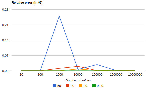
It shows how precision is better for extreme percentiles. The reason why error diminishes for large number of values is that the law of large numbers makes the distribution of values more and more uniform and the t-digest tree can do a better job at summarizing it. It would not be the case on more skewed distributions.
Compression
editApproximate algorithms must balance memory utilization with estimation accuracy.
This balance can be controlled using a compression parameter:
{
    "aggs" : {
        "load_time_outlier" : {
            "percentiles" : {
                "field" : "load_time",
                "compression" : 200
            }
        }
    }
}
The TDigest algorithm uses a number of "nodes" to approximate percentiles — the
more nodes available, the higher the accuracy (and large memory footprint) proportional
to the volume of data. The compression parameter limits the maximum number of
nodes to 20 * compression.
Therefore, by increasing the compression value, you can increase the accuracy of
your percentiles at the cost of more memory. Larger compression values also
make the algorithm slower since the underlying tree data structure grows in size,
resulting in more expensive operations. The default compression value is
100.
A "node" uses roughly 32 bytes of memory, so under worst-case scenarios (large amount of data which arrives sorted and in-order) the default settings will produce a TDigest roughly 64KB in size. In practice data tends to be more random and the TDigest will use less memory.